Linear solver
The heart of a finite element solver is the linear solver, since all equations used to describe the behavior of a structure are finally collected in a single matrix equation of the form
where the vector \(x\) is to be calculated based on a known matrix \(\mathbf{A}\) and the vector \(b\). Two numerical methods exist in general to solve this equation.
Direct solver
Iterative solver
It is very important to understand that a direct solver simply solves the equation without consideration of the nature of the system, while physics plays a role in iterative methods, and particular, their multigrid preconditioners (see below), so it is important for the latter to comprehend the parameters to be used. Anyway, the decision on which solver to use is illustrated in the following flow chart:
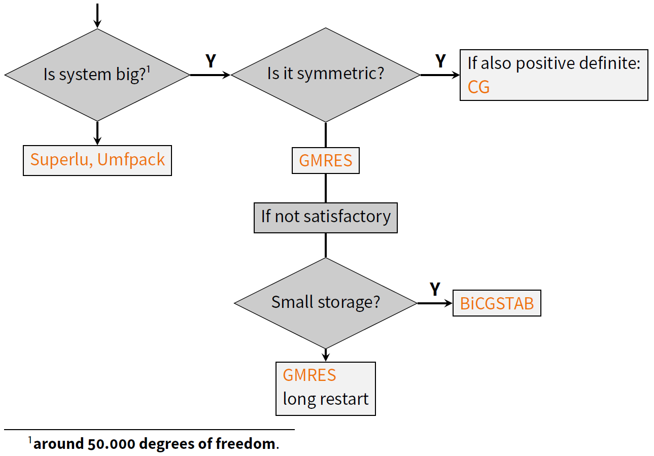
Flowchart of the decision process for an appropriate linear solver, taken from a presentation held by Max Firmbach in 2022.
At this point, the linear algebra library Trilinos is heavily used, which provides a number of packages on different levels:
Sparse linear algebra: Epetra/TPetra
Graph, matrix and vector data structures
Ready for parallel computing on distributed memory clusters
Direct solvers: Amesos/Amesos2
Internal solver implementation (KLU/KLU2)
Interfaces to external solvers (e.g., UMFPACK or Superlu_dist)
Iterative solvers: Belos
Krylov methods (e.g., Conjugate Gradient, GMRES, BiCGStab, and others)
Least squares solvers
One-level domain decomposition and basic iterative methods: Ifpack
Incomplete factorization methods (e.g., ILU, ILUT)
Point relaxation methods (e.g., Jacobi, Gauss-Seidel)
Polynomial methods (e.g., Chebyshev iteration)
Algebraic multigrid methods: MueLu
Construction of algebraic multigrid (AMG) hierarchies
AMG applicable as solver or preconditioner
AMG for single- and multiphysics problems
Block preconditioners: Teko
Block relaxation methods (e.g., block Jacobi, block Gauss-Seidel)
Block factorization methods (e.g., block LU, SIMPLE)
The linear solvers are defined in the solver sections.
Note
All file snippets in this section are presented in the yaml input file format. Consult the documentation for further information, e.g. on converting other input formats to the yaml format.
SOLVER 1:
  SOLVER: "<solver_type>"
  NAME: "<user-defined_solver_name>"
  # further parameters
in which all details for a specific solver are defined; up to 9 solvers can be defined here.
The parameter SOLVER defines the solver to be used.
Most of the solvers require additional parameters. These are explained in the following.
Solvers for single-field problems
When dealing with a single physical field, e.g. solid mechanics, incompressible fluid flow, or heat conduction,
the arising linear system matrix can be tackled by a single linear solver.
In this case, it is sufficient to define a single SOLVER section in the input file.
As an example, consider a solid problem governed by the equations of elasto-dynamcis. To select UMFPACK as direct solver for such a problem, one has to
Define the linear solver: Define the linear solver by adding a
SOLVERsection to the input file and set theSOLVERparameter to"UMFPACK".Assign linear solver to the solid field: Set the
LINEAR_SOLVERparameter in theSTRUCTURAL DYNAMICsection to the ID of the desired linear solver.
An input file could read as follows:
PROBLEM TYPE:
  PROBLEMTYPE: "Structure"
STRUCTURAL DYNAMIC:
  LINEAR_SOLVER: 1
  # further parameters
SOLVER 1:
  SOLVER: "UMFPACK"
Solvers for coupled problems (aka multiphysics)
Partitioned solution using a staggered or iterative coupling scheme:
If a multiphysics problem is to be solved using a partitioned approach, the interaction between the fields is resolved by an iteration between the individual fields. The solution of each individual field is computed by running a nonlinear solver of each single field problem independent of others, which naturally results in linear solvers of each field being independent of each other. Hence, the arising linear systems are always restricted to a single physical field. Each individual physical field of the multiphysics problem is solved like a single physics problems. To this end, one solver has to be assigned to each physics. For convenience, the same definition of a linear solver can be used in multiple physical fields.
For example, a structural analysis sequentially coupled with scalar transport needs two solvers, handling the respective physics:
PROBLEM TYPE:
  PROBLEMTYPE: "Structure_Scalar_Interaction"
STRUCTURAL DYNAMIC:
  LINEAR_SOLVER: 1
  # further parameters
SCALAR TRANSPORT DYNAMIC:
  LINEAR_SOLVER: 2
  # further parameters
SOLVER 1:
  SOLVER: "UMFPACK"
SOLVER 2:
  SOLVER: "UMFPACK"
For the case above, actually, one could also use LINEAR_SOLVER 1 in the section SCALAR TRANSPORT DYNAMIC (and drop the definition of SOLVER 2 entirely).
Monolithic solution:
If a monolithic solution scheme is used, the degrees of freedom of all physical fields are collected in a single vector of unknowns and, thus, result in a single linear system of equations. Given the different nature of the individual fields in a monolithic system, it is not uncommon that the linear system is particularly ill-conditioned.
For the monolithic solution of the multiphysics problem, an additional solver is needed for the monolithic approach, e.g., again for the SSI problem:
PROBLEM TYPE:
  PROBLEMTYPE: "Structure_Scalar_Interaction"
STRUCTURAL DYNAMIC:
  LINEAR_SOLVER: 1
  # further parameters
SCALAR TRANSPORT DYNAMIC:
  LINEAR_SOLVER: 1
  # further parameters
SSI CONTROL/MONOLITHIC:
  LINEAR_SOLVER: 2
  # further parameters
SOLVER 1:
  SOLVER: "UMFPACK"
SOLVER 2:
  SOLVER: "Belos"
  SOLVER_XML_FILE: "gmres_template.xml"
  AZPREC: "AMGnxn"
  AMGNXN_TYPE: "XML"
  AMGNXN_XML_FILE: "ssi_mono_3D_27hex8_scatra_BGS-AMG_2x2.xml"
Here, we have used the same solver type (a direct solver) for each physics (structure and scalar transport), and for the coupling we used an iterative solver (Belos). The situation is similar, when fluid-structure or thermo-structure coupling is employed. The iterative solver used for the coupling is particularly suited for this kind of mathematics, where the coupled degrees of freedom are given in a so-called block structure. The solver settings are explained in detail below.
Special case: Contact
Even though contact does not involve several physics directly, the arising linear system may exhibit similar properties due to the presence of Lagrange multiplier unknowns to enforce the contact constraints.
The following scenarios are covered by 4C:
Contact with penalty: basically still a solid mechanics problem, probably just a bit more ill-conditioned
Contact with lagrange multipliers:
If Lagrange multipliers are kept as unknowns in the linear system, it exhibits a block structure. It is beneficial to tailor the preconditioner to this block structure.
If Lagrange multipliers have been removed from the system through static condensation, the layout of the system does not differ very much from a regular solid mechanics problem. Knowledge about the contact interface might still be beneficial for designing a good preconditioner.
Solver Interfaces
Direct solver
Direct solvers identify the unknown solution \(x\) of the linear system \(Ax=b\) by calculating \(x\) in one step. In modern direct solvers, this usually involves a factorization \(A=LU\) of the system matrix \(A\).
In 4C, we have the following direct solvers available:
UMFPACK, using a multifront approach, thus a sequential solver (can only use a single core)
Superlu_dist, an MPI based solver, which may run on many cores and compute nodes.
Compared to iterative solvers, these solvers do not scale well with the numbers of equations, and are therefore not well suited for large systems. If one has to solve a system with more than 50000 degrees of freedom (approx. equal to number of equations), the iterative solver will be significantly faster. In addition, the iterative solver is more memory efficient, so it can solve larger system with a computer equipped with low memory.
The benefit of the direct solver is that there are no parameters, which one has to provide, since the direct solver does not care about the underlying physics. The definition in the input file is simply
SOLVER 1:
  SOLVER: "UMFPACK"
or
SOLVER 1:
  SOLVER: "Superlu"
Iterative solver
The iterative solver can be used for any size of equation systems, but is the more efficient the larger the problem is. If a good parameter set for the solver is chosen, it scales linearly with the size of the system, either with respect to time or to the number of cores on which the system is solved.
The main drawback is that one has to provide a number of parameters, which are crucial for a fast and correct solution.
Contrary to the direct solver, the matrix must not be factorized. Instead, this solution method solves the equation \(\mathbf{A} x_k = b\) with an initial guess \(x_0 (k=0)\) and an iteration
such that \(x_k \rightarrow x \mbox{ for } k \rightarrow \infty\). Slow progress if \(x_0\) is not chosen properly. A preconditioner helps by solving \(\mathbf{P}^{-1} \mathbf{A} x = \mathbf{P}^{-1} b\). Ideally \(\mathbf{P}^{-1} = \mathbf{A}\) (gives the solution for x), but \(\mathbf{P}\) should be cheap to calculate. The larger the problem is, the higher is the benefit of iterative solvers.
4C’s iterative solvers are based on Trilinos’ Belos package. This package provides a bunch of Krylov solvers, e.g.
CG (conjugate gradient method) for symmetric problems,
GMRES (Generalised Minimal Residual Method), also for unsymmetric problems
BICGSTAB (Biconjugate gradient stabilized method), also for unsymmetric problems
Whether a problem is symmetric or not, depends on the physics involved. The following table gives a few hints:
Problem |
Symmetry |
Remarks |
|---|---|---|
Convection dominated flow |
unsymmetric |
|
elasticity, thermal |
symmetric |
unsymmetric, if Dirichlet boundary conditions are used |
thermal flow |
symmetric |
|
Contact |
unsymmetric |
definitely if friction is involved or Lagrange multiplyers are used |
Iterative solvers are defined via an xml file. The solver section then reads:
SOLVER 2:
  SOLVER: "Belos"
  SOLVER_XML_FILE: "gmres_template.xml"
  # further parameters
Note that the solver itself is always defined as SOLVER: "Belos".
One can find a number of template solver xml files in <source-dir>/tests/input-files/xml/linear_solver/*.xml.
Further parameters are necessary for the preconditioner, where a number of choices are available, see below.
Note
Historically, the parameters for the solver have been defined in the solver sections directly; however, this is deprecated now and we actively migrate to xml-based input of solver parameters.
Preconditioners
The choice and design of the preconditioner highly affect performance. In 4C, one can choose between the following four preconditioners:
ILU
MueLu
Teko
AMGnxn
ILU is the easiest one to use with very few parameters; however, scalability cannot be achieved with this method.
For better performance, especially on large systems, use MueLu for single physics and Teko or MueLu (or AMGnxn) for multiphysics problems.
You’ll find templates of parameter files for various problems in the subdirectories of <source-dir>/tests/input-files/xml/....
The preconditioner is chosen by the parameter AZPREC within the SOLVER n section.
Note that the parameter to define the xml-file for further preconditioner-parameters is different for each preconditioner.
The solver sections appear in the following way:
SOLVER 1:
  NAME: "iterative_solver_with_ILU_preconditioner"
  SOLVER: "Belos"
  SOLVER_XML_FILE: "gmres_template.xml"
  AZPREC: "ILU"
  IFPACK_XML_FILE: "<path/to/your/ifpack_parameters.xml>"
  # template file is located in <source-root>/tests/input-files/xml/preconditioner/ifpack.xml
SOLVER 2:
  NAME: "iterative_solver_with_algebraic_multigrid_preconditioner"
  SOLVER: "Belos"
  SOLVER_XML_FILE: "gmres_template.xml"
  AZPREC: "MueLu"
  MUELU_XML_FILE: "<path/to/your/muelu_parameters.xml>"
  # template files for various problems are located in <source-root>/tests/input-files/xml/multigrid/*.xml
SOLVER 3:
  NAME: "iterative_solver_with_block_preconditioner"
  SOLVER: "Belos"
  SOLVER_XML_FILE: "gmres_template.xml"
  AZPREC: "Teko"
  TEKO_XML_FILE: "<path/to/your/teko_parameters.xml>"
  # template files for various problems are located in <source-root>/tests/input-files/xml/block_preconditioner/*.xml
SOLVER 4:
  SOLVER: "Belos"
  AZPREC: "AMGnxn"
  SOLVER_XML_FILE: "gmres_template.xml"
  NAME: "iterative_solver_with_AMGnxn_preconditioner"
  AMGNXN_TYPE: "XML"
  AMGNXN_XML_FILE: "<path/to/your/amgnxn_parameters.xml>"
  # template files for various problems are located in <source-root>/tests/input-files/*AMG*.xml
The xml template files (see the comments in the respective solver sections) are named after problem types for which they are most suited. It is highly recommended to first use these defaults before tweaking the parameters.
ILU (incomplete LU method) comes with a single parameter, therefore only a single xml file is contained in the respective directory:
<source-dir>/tests/input-files/xml/preconditioner/ifpack.xml.
In this file, the so-called fill level is set up by fact: level-of-fill, and it contains the default value 0 there.
With lower values, the setup will be faster, but the approximation is worse.
The higher the more elements are included, sparcity decreases (a level of 12 might be a full matrix, like a direct solver).
The current recommendation is to use one of the three more sophisticated preconditioners available. All these preconditioners have a number of parameters that can be chosen; however, a recommended set of parameters for various problems are given in respective xml files.
In general, the xml file for the multigrid preconditioners usually contains the divisions
general
aggregation
smoothing
repartitioning
For preconditioning of large systems, the trick is to apply a cheap transfer method to get from the complete system to a smaller one (coarsening/aggregation of the system). Here, coarsening means the generation of a smaller system size, will aggregation is the reverse procedure to come to the original matrix size. The coarsening reduces the size by comprised a number of lines into one; common choices are 27 for 3D, 9 for 2D, and 3 for 1D problems, which is conducted by default.
The overall multigrid algorithm is defined in the general section by multigrid algorithm, which can have the values
sa (Classic smoothed aggregation, default), pg (prolongator smoothing) among others.
A smoother is used twice (pre- and post-smoother) for each level of aggregation to reduce the error frequencies in your solution vector.
Multiple transfer operations are applied in sequence, since only high frequency components can be tackled by smoothing,
while the low frequency errors are still there.
The restriction operator restricts the current error to the coarser grid.
At some point (let say if 10000 dofs are left) the system has a size where one can apply the direct solver.
This number is given by coarse:: max size in the general section of the xml file.
That is, when the number of remaining dofs is smaller than the given size, no more coarsening is conducted.
It should be larger than the default of 1000, let say, 5000-10000.
Also, the maximum number of coarsenings is given by max levels. This number should always be high enough to get down to the max size, the default is 10.
After reaching the coarsest level, the remaining system is solved by a (direct) solver.
The parameter to setup the direct solver is coarse: type,
and it can have the values SuperLU (default), SuplerLU_dist (the parallel version of SuperLU), KLU (an internal direct solver in trilinos) or Umfpack.
(After changing to Amesos2, the internal server will be KLU2).
The smoother to be used is set up by smoother: type with the possible values CHEBYSHEV, RELAXATION (default), ILUT, or RILUK
While many solvers can be used, five of them are most popular: SGS (symmetric Gauss Seidel), Jacobi, Chebyshev, ILU, MLS.
Besides that, particularly for the coarsest smoother, a direct solver can be used, as (Umfpack, SuperLU, KLU).
- Chebyshev smoother:
This is a polynomial smoother. The degree of the polynomial is given by smoother: sweeps (default is 2). A lower degree is faster (not much), but higher is more accurate; reasonable values may go up to 9 (very high)
- Relaxation method:
The relaxation smoother comes with a number of additional parameters inside a special section , particularly the type:
relaxation: type, which can beJacobi,Gauss-Seidel,Symmetric Gauss-Seidelamong others. The polynomial degree can be setup here byrelaxation: sweeps. This one is rather for fluid dynamics problems.- ILUT, RILUK:
These are local (processor-based) incomplete factorization methods.
For understanding the multigrid preconditioner better, the interested reader is referred to a presentation held by Max Firmbach in 2022.
Damping helps with convergence, and it can be applied to any of the smoothers by smoother: damping factor.
A value of 1 (default) cancels damping, 0 means maximum damping.
Too much damping increases the iterations, thus, usually it should be between 1 and 0.5.
A little bit of damping will probably improve convergence (also from the beginning).
For the multigrid preconditioner, one can also find a comprehensive documentation
on the trilinos website, explaining all the parameters, their meaning and the default values.