FSI Tutorial 2d with pre_exodus and Cubit
Introduction
As example, we consider a 2d driven cavity example as sketched in Fig. 1.1. For further details and references we refer the reader to [Wall99]
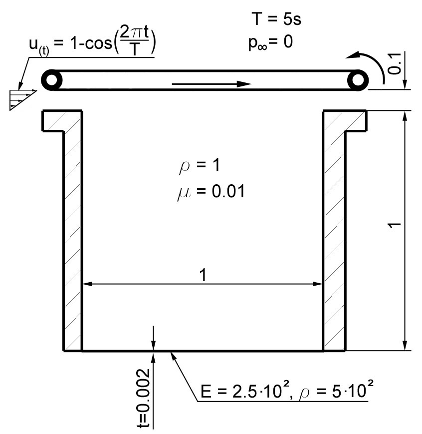
The driven cavity example in 2d
You can find the complete journal file within your 4C distribution. It is located in <4C-sourcedir>/tests/framework-test/tutorial_fsi.jou.
Within Cubit, open the Journal-Editor (Tools\(\to\)Journal Editor), paste the text from the journal file and press play.
Export now the created geometry and mesh to an exodus-file (filename: dc2d.exo) via File\(\to\)Export…. During export, set the dimension explicitly to 2d.
General Procedure of Creating a Valid 4C Input File
With a given mesh including some nodal clouds to apply conditions to you need another text-file (bc-file) where you specify, what you would like to do with it. It contains for example the specific element declaration (fluid, structure, parameters, etc.) and the particular boundary condition such as Dirichlet or Neumann. Finally, a header-file consists of general parameters such as solvers, algorithmic parameters, etc. Those three files are merged by pre_exodus into an input file for 4C. This file is then automatically validated using all available 4C validation and is therefore likely to run.
Sure, you usually do not have already a proper header-file and matching bc-file. By typing
./pre_exodus --exo=yourmesh.e
you get two preliminary files ’default.head’ and ’default.bc’. The first contains the currently valid header parameters with default values and commented options which you can edit to adapt it to your means. Similarly, ’default.bc’ consists of all your mesh entities and a list of all currently valid conditions. See next section for details how to work with it and how to get valid input files.
Running a Simulation with 4C
To start the solver use the call
./4C [inputdirectory]/your_example.dat [outputdirectory]/outputprefix
(in the 4C-directory; of course, you may choose a different directory as well, if you take care for the path names). The results are then written to the result directory with the prefix you chose.
The FSI problem with a partitioned solver
Here, we create the 4C input file for the FSI problem, that is solved using a partitioned scheme, which means that the fluid and the solid problem are solved sequentially. For a monolithic scheme, see the section below.
After running the 4C executable without boundary condition and header information, we have created the ’default.head’ and ’default.bc’ file` that we are now supposed to edit.
header-file
Find the following sections in ’default.head’ and edit as given:
ALE DYNAMICLINEAR_SOLVER 1FLUID DYNAMICCONVTOL 1e-08GRIDVEL BDF2ITEMAX 50LINEAR_SOLVER 2TIMEINTEGR Np_Gen_AlphaFSI DYNAMICMAXTIME 3NUMSTEP 30SECONDORDER yesSHAPEDERIVATIVES yesTIMESTEP 0.1SOLVER 1NAME ALE solverSOLVER UMFPACKSOLVER 2NAME Fluid solverSOLVER Aztec_MSRSOLVER 3NAME Structure solverSOLVER UMFPACKSTRUCTURAL DYNAMICLINEAR_SOLVER 3TOLRES 1e-10MATERIALSinsert
MAT 1 MAT_fluid DYNVISCOSITY 0.01 DENSITY 1.0for definition of fluid materialinsert
MAT 2 MAT_ElastHyper NUMMAT 1 MATIDS 3 DENS 500to define a hyperelastic structural materialinsert
MAT 3 ELAST_CoupNeoHooke YOUNG 250.0 NUE 0.0to specify the structural material as Neo-Hooke materialinsert
MAT 4 MAT_Struct_StVenantKirchhoff YOUNG 1.0 NUE 0.0 DENS 1.0to define an ALE materialCLONING MATERIAL MAPinsert
SRC_FIELD fluid SRC_MAT 1 TAR_FIELD ale TAR_MAT 4to specify the ALE material that is used for the fluid fieldFUNCT 1insert
SYMBOLIC_FUNCTION_OF_SPACE_TIME (1-cos(2*t*pi/5))defining time-dependent inflow and lid movementFUNCT 2insert
SYMBOLIC_FUNCTION_OF_SPACE_TIME 10*(y-1)*(1-cos(2*t*pi/5))representing the spatial inflow distribution
Safe the file under a different name, e.g. ’dc2d_fsi.head’.
bc-file
The main section of the default.bc file contains the element set and boundary condition information:
--------------------------BCSPECS

Element Block, named:
of Shape: HEX8
has <xxx> Elements
*eb1="ELEMENT"
sectionname=""
description=""
elementname=""

[further element sections]

Node Set, named: <bc_name>
Property Name: none
has <xx> Nodes
*ns1="CONDITION"
sectionname=""
description=""

[further node set definitions to be used for conditions]
Edit the ’default.bc’ file as follows:
For the element definitions, which are consecutively enumerated as eb<number>:
*eb1="ELEMENT"the structure elements with their materialsectionname="STRUCTURE" description="MAT 2 KINEM nonlinear EAS none THICK 1.0 STRESS_STRAIN plane_strain GP 2 2" elementname="WALL"
*eb2="ELEMENT"the fluid elements with ALE and the fluid materialsectionname="FLUID" description="MAT 1 NA ALE" elementname="FLUID"
For Dirichlet boundary conditions for structure, fluid and ALE, which are defined by a node set number, ns<number>, but also by its name:
*ns1="CONDITION"Fixing the structure at left and right sidesectionname="DESIGN LINE DIRICH CONDITIONS" description="NUMDOF 2 ONOFF 1 1 VAL 0.0 0.0 CURVE none none FUNCT 0 0"
*ns2="CONDITION"sectionname="DESIGN FSI COUPLING LINE CONDITIONS" description="coupling_id 1"
*ns3="CONDITION"sectionname="DESIGN POINT DIRICH CONDITIONS" description="NUMDOF 2 ONOFF 1 1 VAL 0.0 0.0 CURVE none none FUNCT 0 0"
*ns4="CONDITION"sectionname="DESIGN POINT DIRICH CONDITIONS" description="NUMDOF 2 ONOFF 1 1 VAL 0.0 0.0 CURVE none none FUNCT 0 0"
*ns5="CONDITION"sectionname="DESIGN LINE DIRICH CONDITIONS" description="NUMDOF 3 ONOFF 1 1 0 VAL 0.0 0.0 0.0 CURVE none none none FUNCT 0 0 0"
*ns6="CONDITION"sectionname="DESIGN LINE DIRICH CONDITIONS" description="NUMDOF 3 ONOFF 1 1 0 VAL 1.0 0.0 0.0 CURVE 1 none none FUNCT 0 0 0"
*ns7="CONDITION"sectionname="DESIGN LINE DIRICH CONDITIONS" description="NUMDOF 3 ONOFF 1 1 0 VAL 1.0 0.0 0.0 CURVE 1 none none FUNCT 1 0 0"
*ns8="CONDITION"sectionname="DESIGN LINE ALE DIRICH CONDITIONS" description="NUMDOF 2 ONOFF 1 1 VAL 0.0 0.0 CURVE none none FUNCT 0 0"
*ns9="CONDITION"sectionname="DESIGN FSI COUPLING LINE CONDITIONS" description="coupling_id 1"
*ns10="CONDITION"sectionname="DESIGN POINT DIRICH CONDITIONS" description="NUMDOF 3 ONOFF 1 1 0 VAL 1.0 0.0 0.0 CURVE 1 none none FUNCT 0 0 0"
*ns11="CONDITION"sectionname="DESIGN POINT DIRICH CONDITIONS" description="NUMDOF 3 ONOFF 1 1 0 VAL 0.0 0.0 0.0 CURVE none none none FUNCT 0 0 0"
*ns12="CONDITION"sectionname="DESIGN POINT DIRICH CONDITIONS" description="NUMDOF 3 ONOFF 1 1 0 VAL 0.0 0.0 0.0 CURVE none none none FUNCT 0 0 0"
*ns13="CONDITION"sectionname="DESIGN POINT ALE DIRICH CONDITIONS" description="NUMDOF 2 ONOFF 1 1 VAL 0.0 0.0 CURVE none none FUNCT 0 0"
Copy the following condition and parametrize it as given below to further prescibe Dirichlet boundary conditions on the ALE field:
*ns6="CONDITION"sectionname="DESIGN LINE ALE DIRICH CONDITIONS" description="NUMDOF 2 ONOFF 1 1 VAL 0.0 0.0 CURVE none none FUNCT 0 0"
As any of these conditions matches an already defined NodeSet it will also match the corresponding ’E-id’ in the later 4C input file. Finally save the file under a different name, e.g. ’dc2d_fsi.bc’.
Creating 4C Input File and Running the Simulation
Run in a shell
 ./pre_exodus --exo=dc2d.e --head=dc2d_fsi.head
--bc=dc2d_fsi.bc --dat=dc2d_fsi.dat
where the filenames might have to be replaced accordingly.
This will result in the specified dat-file which is already validated to be accepted by 4C.
However, if the file is meaningful cannot be assured.
Hint: When you have an already existing input file, you can always
validate it by simply executing ./pre_exodus --dat=inputfile.dat,
before(!) you start a parallel 4C computation on a cluster, for
example.
Run the simulation by providing the created dat-file and an output file to 4C and postprocess the results.
Postprocessing
You can postprocess your results with any visualization software you like. In this tutorial, we choose Paraview.
Before you can open the results, you have to generate a filter again. Call make post_drt_ensight in the 4C-directory. Filter your results in the output directory with the call
./post_drt_ensight --file=[outputdirectory]/outputprefix
After this open paraview, go to
File:math:`to`Open Data and select the filtered *.case file.
Only for older versions of Paraview:
Select the time step in the Select Time Value window on the left and
shift Byte order to little endian
Click on accept (or apply) to activate the display.
In the Display tab (section Color) you can choose now between Point pressure and Point velocity, whatever you want to display.
Use a warp vector to visualize the simulation results on the deformed domain.
For the scale, activate the Scalar bar button in the View section.
The FSI problem with a monolithic solver
There are two possibilities for monolithic schemes:
fluid-split: the fluid field is chosen as slave field, the structure field is chosen as master field.
structure-split: the structure field is chosen as slave field, the fluid field is chosen as master field.
In order to use a monolithic solver, change the coupling algorithm
COUPALGO in the FSI DYNAMIC section in the *.head-file.
Additionally, special care has to be taken of the interface degrees of
freedom, that are subject to Dirichlet boundary conditions. The
interface is always governed by the master field. The slave interface
degrees of freedom do not occur in the global system of equations and,
thus, are not allowed to carry Dirichlet boundary conditions.
Tolerances for the nonlinear convergence check in monolithic FSI are set
with the following parameters in the FSI DYNAMIC section:
TOL_DIS_INC_INFTOL_DIS_INC_L2TOL_DIS_RES_INFTOL_DIS_RES_L2TOL_FSI_INC_INFTOL_FSI_INC_L2TOL_FSI_RES_INFTOL_FSI_RES_L2TOL_PRE_INC_INFTOL_PRE_INC_L2TOL_PRE_RES_INFTOL_RPE_RES_L2TOL_VEL_INC_INFTOL_VEL_INC_L2TOL_VEL_RES_INFTOL_VEL_RES_L2fluid split
Choose
iter_monolithicfluidsplitasCOUPALGOin theFSI DYNAMICsection.Modify Dirichlet condition
*ns12="CONDITION"tosectionname="DESIGN POINT DIRICH CONDITIONS" description="NUMDOF 3 ONOFF 0 0 0 VAL 0.0 0.0 0.0 CURVE none none none FUNCT 0 0 0"
in order to remove the Dirichlet boundary conditions from the fluid (=slave) interface degrees of freedom.
Create the input file as described above. Start 4C as usual.
structure split
Choose
iter_monolithicstructuresplitasCOUPALGOin theFSI DYNAMICsection.Modify Dirichlet condition
*ns4="CONDITION"tosectionname="DESIGN POINT DIRICH CONDITIONS" description="NUMDOF 2 ONOFF 0 0 VAL 0.0 0.0 CURVE none none FUNCT 0 0"
in order to remove the Dirichlet boundary conditions from the structure (=slave) interface degrees of freedom.
Create the input file as described above. Start 4C as usual.