3D Solid Tutorial with Coreform Cubit® and pre_exodus

Introduction

This tutorial gives an introduction to the usage of 4C for simulating plastic material behaviour. It is assumed that 4C including the pre-processing tool pre_exodus has been built on your machine according to the instructions and has passed the tests without error messages. In addition, the pre-processing of the finite element model is built with Coreform Cubit, but the input file can also be generated without this software.

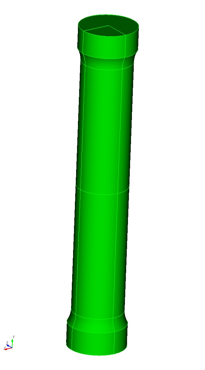
The analyzed structure is a simple round tensile bar, which is commonly used to identify the material’s stress-strain curve by comparing the simulation with the respective experiment. The geometry, which has a cross sectional diameter of 10 mm and a length of constant diameter of 50 mm is shown in the following figure:

Problem definition and geometrical setup

The material under consideration is an Aluminum alloy with a yield strength of 330 MPa and a mild isotropic hardening. During the test, a force F acts on the top of the rod such that it elongates.

For elasto-plastic simulations 4C provides mainly the following seven material models:

MAT_Struct_PlasticLinElast
MAT_Struct_PlasticNlnLogNeoHooke
MAT_Struct_ThermoPlasticHyperElast
MAT_Struct_ThermoPlasticLinElast
MAT_Struct_Damage
MAT_Struct_PlasticGTN
MAT_Struct_DruckerPrager

The following flow chart depicts for which cases these seven models are applicable:

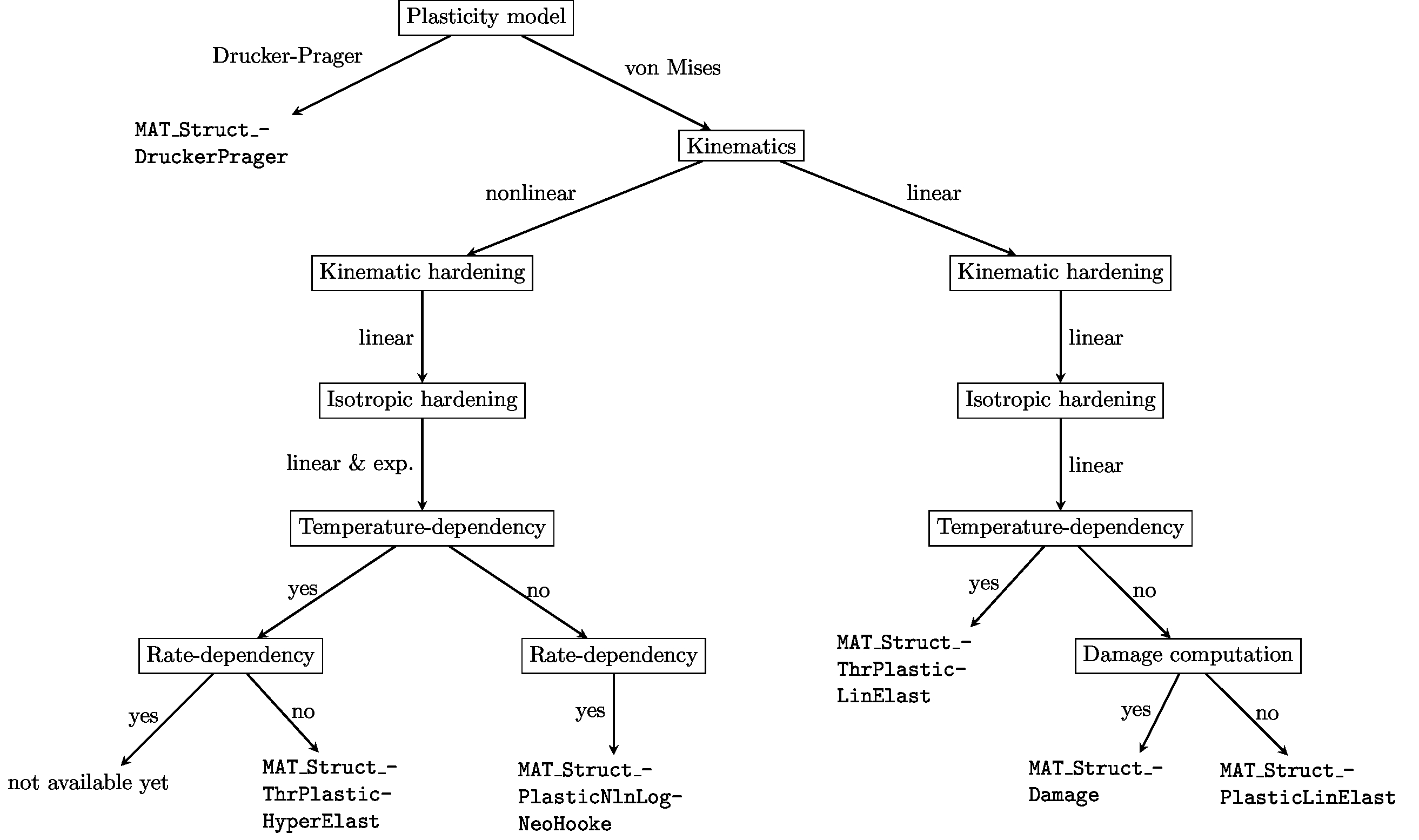
Capabilities of plasticity models available in 4C

Preprocessing

Due to the symmetry of this model, we may restrict our analysis to one half in longitudinal direction. In addition, one can see that the structure has a rotational symmetry. Since axisymmetric elements are not available in 4C, a 3D structure is modelled with double symmetry in both lateral directions, so that only one eighth of the structure is left. The final FE model is shown here.

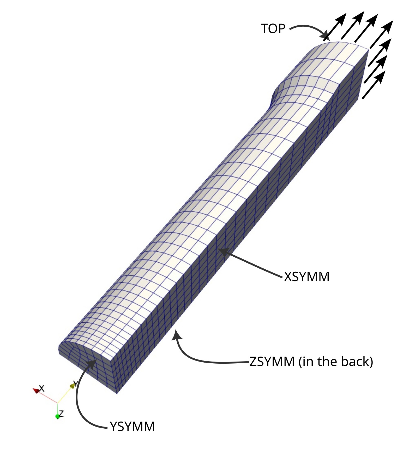
Mesh of one eighth of the tensile bar

Symmetry boundary conditions are applied to the three symmetry planes, denoted with XSYMM, YSYMM, ZSYMM in the above figure. The top surface is subject to a Dirichlet boundary condition with linearly increasing displacement in y-direction.

To this end, we model 200 time steps spanning from \(t_0 = 0\) s to \(t_1 = 1\) s with a time step of \(\Delta t = 0.005\) s. Assuming nonlinear kinematics (large strain theory) and plasticity with isotropic hardening following an exponential curve, namely \(\sigma_Y = \sigma_{Y,0} + (\sigma_{Y,\infty} - \sigma_{Y_0}) \left[ 1 - \exp \left( - k \, \varepsilon_p \right) \right]\) with \(\sigma_{Y,0}=330, \sigma_{Y,\infty} = 1000, k=5\) .

We choose the model MAT_Struct_PlasticNlnLogNeoHooke to accomplish this task, which is a plasticity model that uses von Mises yield criterion

\[\Phi = \tilde{\mathbf{\tau}} - \sqrt{\frac{2}{3}} \sigma_Y\]

with \(\tilde{\mathbf{\tau}}\) being the deviatoric Kirchhoff stress. Additionally, a compressible Neo-Hooke elasticity model expressed by the free energy potential

\[\rho_0 \Psi(\mathbf{B}^e) = \frac{K}{2} \left[ \frac{1}{2} (J^2 - 1) - \ln J \right] + \frac{1}{2} \mu \left[ \text{tr} \mathbf{\tilde{B}}^e - 3 \right]\]

Here, \(J\) is the determinant of the deformation gradient \(\mathbf{F}\), \(\mathbf{B}^e = \mathbf{F}^e {\mathbf{F}^e}^T\) is the elastic part of the left Cauchy Green tensor, and \(K, \mu\) are elastic constants.

The geometry, finite element mesh and node sets for the boundary conditions are created using Coreform Cubit®. The mesh is rather fine and 27-node brick elements have been used herein. The corresponding journal file can be run to reproduce this mesh and output a binary exodus mesh information file tutorial_solid.e. The geometry dimensions (actually mainly the radius, all other dimensions depend on it) and element size can be varied, since they are parametrized in the journal file.

# ===============
# ||  VARIABLES   ||
# ===============
# { radius = 5.0 }
# { elsize_fine = 0.8}   # for higher accuracy, choose 0.4
# { elsize_coarse = 2.5 }
# { total_height = radius*6.5 }
# { head_width = radius*(1+(1-cosd(30))) }
# { coarseness = 6 }   must be between 1 and 9, default 5 is appropriate, 6 is faster, but still okay.

# ================
# ||  GEOMETRY  ||
# ================
# 2D shape
create surface rectangle width {radius}  height {5*radius} zplane
move surface 1 x {radius/2.0} y {radius*2.5} include_merged
create curve arc radius {radius} center location {2*radius} {5*radius} 0 normal 0 0 1 start angle 150 stop angle 180
create curve location 0 {5*radius} 0 location 0 {5*head_width} 0
create curve vertex 5 8
create surface curve 1 5 7 6
create curve location 0 {total_height} 0 location {head_width} {total_height} 0
create surface vertex 8 5 12 11
imprint tolerant surface 1 3 2
merge surface all

# quarter 3D
create curve arc radius {radius} center location 0 0 0 normal 0 1 0 start angle 0 stop angle 90
create curve vertex 3 18
create surface curve 3 14 15
sweep curve 4 5 11  yaxis angle 90
create curve vertex 29 11
create surface curve 28 12 29
create surface curve 29 25 21 17 15 2 6 13
create volume surface all heal
volume 9 redistribute nodes off
volume 9 scheme Sweep source surface 4 target surface 8 sweep transform least squares
volume 9 autosmooth target on fixed imprints off smart smooth off

# ===============
# ||  MESHING  ||
# ===============
curve 17 scheme bias fine size {elsize_fine} coarse size {elsize_coarse} start vertex 18
curve 2 scheme bias fine size {elsize_fine} coarse size {elsize_coarse} start vertex 3
curve 4 scheme bias fine size {elsize_fine} coarse size {elsize_coarse} start vertex 4
curve 25 13 11 interval 2
curve 25 13 11 scheme equal
curve 21 6 5 interval 3
curve 21 6 5 scheme equal
volume 9 size auto factor {coarseness}
mesh volume 9

# =================
# ||  NODE SETS  ||
# =================
nodeset 1 add surface 4
nodeset 1 name "YSYMM"
nodeset 2 add surface 1 2 3
nodeset 2 name "ZSYMM"
nodeset 3 add surface 9
nodeset 3 name "XSYMM"
nodeset 4 add surface 8
nodeset 4 name "TOP"

# ======================
# ||  DUMMY MATERIAL  ||
# ======================
set duplicate block elements off
block 1 add volume 9
block 1 element type hex27
create material "metal" property_group "CUBIT-ABAQUS"
modify material "metal" scalar_properties "MODULUS" 7e+04 "POISSON" 0.33
block 1 material 'metal'

# ====================
# ||  WRITE EXODUS  ||
# ====================
export mesh "tutorial_solid.e"  overwrite

The general definition of the geometry in this cubit journal file, which can be run from the directory <source-root>/tests/framework-test/ includes the complete mesh and four surface node sets. If you don’t have Coreform Cubit, you may use the resulting exodus file directly, which is also located in this directory.

The boundary conditions and loading, the material and all solver details are defined in two other files: A so-called boundary condition file tutorial_solid.bc and a header file tutorial_solid.head. These three files together can be combined to a 4C input file using the command

<build-dir>/pre-exodus --exo=tutorial_solid.e --bc=tutorial_solid.bc --head=tutorial_solid.head

Note that you need to build the pre_exodus command before. You’ll find the build information for pre_exodus in the setup section or in the workflow/preprocessing section.

The boundary condition file tutorial_solid.bc contains the element information and boundary conditions. The element type is a quadratic (27 node) 3D solid element(Solid HEX27) with nonlinear kinematics, that is, including a large strain formulation. The boundary conditions include three symmetry conditions (based on the surfaces defined in Cubit) and one loading condition. Note that only surface conditions are given; the lines that belong to two surfaces automatically get the combined boundary conditions. The loading condition has a function number (1) included for the y-direction, and also gets a tag: TAG monitor_reaction. The tag is for an extra output of the total forces, which are printed in a csv file, if the output is requested.

----------- Mesh contents -----------

Mesh consists of 1598 Nodes, 1155 Elements, organized in
1 ElementBlocks, 4 NodeSets, 0 SideSets

------------------------------------------------BCSPECS

Element Block, named:
of Shape: HEX27
has 1155 Elements
*eb1="ELEMENT"
sectionname="STRUCTURE"
description="MAT 1 KINEM nonlinear"
elementname="SOLID"

Node Set, named: centerplane
Property Name: none
has 47 Nodes
*ns1="CONDITION"
sectionname="DESIGN SURF DIRICH CONDITIONS"
description="NUMDOF 3 ONOFF 0 1 0  VAL 0 0 0 FUNCT 0 0 0  TAG none "

Node Set, named: zsymm
Property Name: none
has 238 Nodes
*ns2="CONDITION"
sectionname="DESIGN SURF DIRICH CONDITIONS"
description="NUMDOF 3 ONOFF 0 0 1  VAL 0 0 0 FUNCT 0 0 0  TAG none "

Node Set, named: xsymm
Property Name: none
has 238 Nodes
*ns3="CONDITION"
sectionname="DESIGN SURF DIRICH CONDITIONS"
description="NUMDOF 3 ONOFF 1 0 0  VAL 0 0 0 FUNCT 0 0 0  TAG none "

Node Set, named: top
Property Name: none
has 47 Nodes
*ns4="CONDITION"
sectionname="DESIGN SURF DIRICH CONDITIONS"
description="NUMDOF 3 ONOFF 0 1 0  VAL 0 1 0 FUNCT 0 1 0  TAG monitor_reaction "

All control parameters for the material, solvers, loading function, output information are contained in tutorial_solid.head. Particularly, the output of the forces is requested by a particular section, IO/MONITOR STRUCTURE DBC, which controls accuracy and frequency of the output. This and all other output information is given in section IO and its subsections.

  DYNAMICTYPE: "Statics"
  RESTARTEVERY: 1000
  NUMSTEP: 10
  MAXTIME: 10
  TOLDISP: 0.0001
  TOLRES: 0.0001
  NORM_RESF: "Rel"
  PREDICT: "TangDis"
  LINEAR_SOLVER: 1
SOLVER 1:
  SOLVER: "Superlu"
  NAME: "Direct_Solver"
SOLVER 2:

You’ll find two solver sections in there. In the original header file, which are selected in the section STRUCTURAL DYNAMIC by the parameter LINEAR_SOLVER. The value of this parameter refers to the section SOLVER x, in which x is the number of the selected solver. In the section SOLVER 1, the direct solver is defined, it does not have any parameters (except an optional name). The iterative solver in section SOLVER 2 has some parameters, namely an xml file, which contains more parameters. The given xml file as well as some other examples for different multiphysics problems are given in the folder <source-root>/tests/input-files/xml/*/*.xml.

  SOLVER: "Belos"
  AZPREC: "MueLu"
  AZTOL: 1e-05
  AZOUTPUT: 1000
  AZSUB: 100
  MUELU_XML_FILE: "elasticity_template.xml"
  NAME: "Iterative_Solver"
MATERIALS:
  - MAT: 1
    MAT_Struct_PlasticNlnLogNeoHooke:
      YOUNG: 70000
      NUE: 0.33
      DENS: 1
      YIELD: 330
      SATHARDENING: 1000
      HARDEXPO: 5
      VISC: 0.01
      RATE_DEPENDENCY: 1
FUNCT1:
  - COMPONENT: 0
    SYMBOLIC_FUNCTION_OF_SPACE_TIME: "pull"
  - VARIABLE: 0
    NAME: "pull"
    TYPE: "linearinterpolation"
    NUMPOINTS: 2
    TIMES: [0,20]
    VALUES: [0,20]
RESULT DESCRIPTION:
  - STRUCTURE:
      DIS: "structure"
      NODE: 2477
      QUANTITY: "dispy"
      VALUE: 0.4561235910743636
      TOLERANCE: 1e-12

If you choose LINEAR_SOLVER  2, you’ll get the iterative solver. Note that you have to copy the xml file to your folder before executing pre_exodus with the iterative solver setting.

The STRUCTURAL DYNAMIC section also defines the time integration, particularly the time stepping. Time step size is given by TIMESTEP, the maximum time is given by MAXTIME and the maximum number of increments is NUMSTEP. The end of the simulation is defined either when the maximum time or when the number of increments is reached, whatever comes earlier. Note that the number of time steps is currently set to 10, in order to keep the simulation time short for the CI/CD tests. If you want to run the whole simulation including necking of the specimen, you have to change the parameter to at least NUMSTEP 200.

Besides output and solver details, the material and any functions are defined in the header. For the material, we choose a large strain plasticity model, which is named MAT_Struct_PlasticNlnLogNeoHooke with parameters, which might represent a high strength Aluminum. Last but not least, a function is defined in this file, to which the Dirichlet boundary condition refers.

      NAME: "elongation"
  - STRUCTURE:
      DIS: "structure"
      NODE: 6
      QUANTITY: "dispx"

Simulation

After the file tutorial_solid.dat has been created successfully using the pre_exodus command shown above, the simulation is run on a single processor by the command

<build-dir>/4C tutorial_solid.dat tutorial_solid

Since the solver output is quite lengthy, one might want to redirect it into a file. For running the simulation with several processes, use mpirun -np <n_cpu> <build-dir>/4C [further parameters].

Post processing

The VTK results are collected in the directory tutorial_solid-vtk-files/. If they shall be opened by Paraview, the data file tutorial_solid-structure.pvd contains the complete collection of files, so only this file is to be opened, all other files are then read automatically. Using the filter Warp by vector with Coloring defined by the scalar accumulated_plastic_strain, one may obtain a contour plot on the deformed geometry:

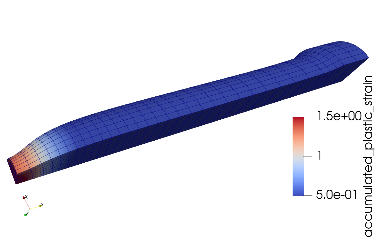
Deformed mesh with contours of accumulated plastic strain

The output of the forces needed to apply the Dirichlet boundary condition are given in the directory tutorial_solid_monitor_dbc. Each boundary condition using the tag monitor_reaction creates a single ASCII file with suffix .csv, which for the present case provides the time, the force in y-direction and the initial and current area to which the force is applied. Since the displacement itself is not given in this file, the displacement is to be calculated from the time.

A force-displacement graph may be created using gnuplot by the lines

set terminal png size 1200,900 font Arial 14
set output 'tutorial_solid_graph.png'
set key off
set xlabel "displacement"; set ylabel "force"; set title "Force-displacement curve"
plot "tutorial_solid_monitor_dbc/tutorial_solid_10004_monitor_dbc.csv" using ($2*12):(abs($6))  with lines title "force-displacement"

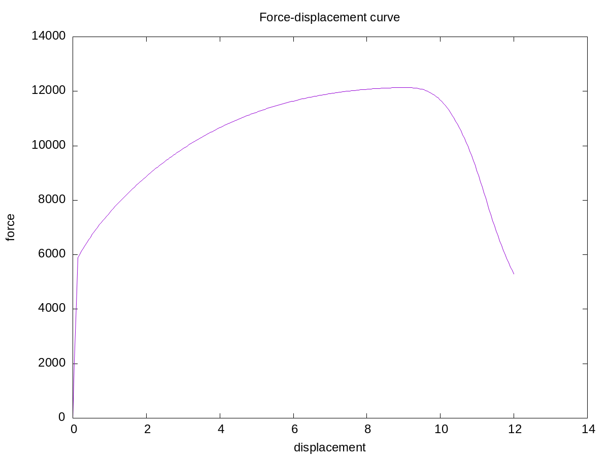
Force displacement curve for the tensile bar