Fluid Tutorial with pre_exodus and Cubit
For this as for all other tutorials you’ll need a complete 4C installation as well as access to the pre-processing tool cubit and the post-processing tool paraview. If you did not do so already, install 4C based on the information given in the Installation Guide.
Introduction
In this tutorial we want to simulate the incompressible flow past a circular cylinder. For further details and references we refer the reader to: [Wall99]
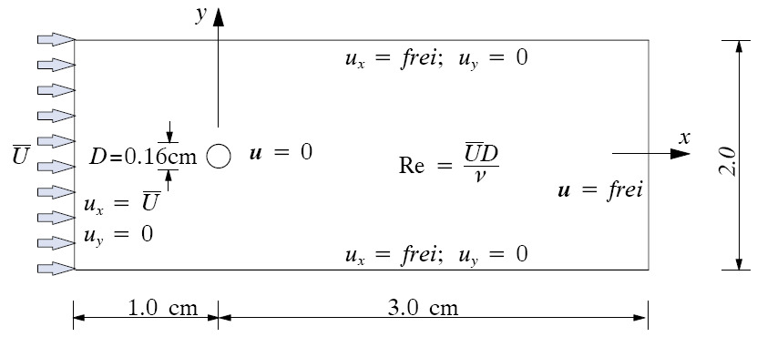
Problem definition and geometrical setup (with friendly permission ;-))
Preprocessing
Creating the Geometry with Cubit
We will use Cubit for creating the geometry and the mesh.
Within Cubit, open the Journal-Editor (Tools \(\to\) Journal
Editor), paste the text below and press play. If the geometry
couldn’t be created, try to set the editor to ’Translate to Cubit
commands’ first and retry. Alternatively, double-check every single line
of the text, since sometimes errors occur during copying and pasting.
After successful geometry and mesh creation, export everything to an
Exodus-file of your choice via File \(\to\)Export…. Select
the folder build-release created before, pick an arbitrary name for
the file, click on Save, and then set the dimension explicitly to
2d.
 1$***********************
 2$ preliminaries
 3$***********************
 4reset
 5set geometry engine acis
 6$***********************
 7$ create geometry
 8$***********************
 9
10$ define geometric parameters
11$ in cm
12# {fluid_length = 4.0} $ x-direction
13# {fluid_width = 2.0} $ y-direction
14# {cyl_radius = 0.08}
15# {cyl_offset = 1.0}
16$ create domain
17create vertex {-cyl_offset} {fluid_width/2.0} 0
18create vertex {-cyl_offset} {-fluid_width/2.0} 0
19create vertex {fluid_length-cyl_offset} {fluid_width/2.0} 0
20create vertex {fluid_length-cyl_offset} {-fluid_width/2.0} 0
21create vertex 0 0 0
22create vertex {cyl_offset} {fluid_width/2.0} 0
23create vertex {cyl_offset} {-fluid_width/2.0} 0
24create curve vertex 1 vertex 5
25create curve vertex 5 vertex 6
26create curve vertex 6 vertex 1
27create curve vertex 10 vertex 2
28create curve vertex 2 vertex 8
29create curve vertex 12 vertex 7
30create curve vertex 7 vertex 13
31create curve vertex 15 vertex 9
32create curve vertex 18 vertex 3
33create curve vertex 3 vertex 4
34create curve vertex 4 vertex 17
35create surface curve 3 1 2
36create  surface curve 1 4 5
37create  surface curve 5 6 7
38create  surface curve 7 8 2
39create  surface curve 8 9 10 11
40create vertex 0 0 0
41create vertex 0 {cyl_radius} 0
42create vertex {cyl_radius} 0 0
43create curve arc center vertex 24 25 26 {cyl_radius} full
44create surface curve 17
45delete vertex 24 25 26
46subtract volume 6 from volume 1 2 3 4
47imprint volume all
48merge volume all
49
50$***********************
51$ create mesh
52$***********************
53
54# {numele_past_x = 37}
55# {numele_past_y = 34}
56# {numele_cyl_x = 30}
57# {numele_inflow = 22}
58# {numele_radial = 50}
59group "radial" add curve 19 20 23 26
60curve  9 scheme equal interval {numele_past_x}
61curve  10 scheme equal interval {numele_past_y}
62curve  in group radial scheme equal interval {numele_radial}
63curve  3 6 scheme equal interval {numele_cyl_x}
64curve  4 scheme equal interval {numele_inflow}
65$ apply bias for better mesh
66curve 19 scheme bias factor 0.9 start vertex 1 interval {numele_radial}
67propagate curve bias volume all
68curve 20 scheme bias factor 0.9 start vertex 6 interval {numele_radial}
69propagate curve bias volume all
70curve 23 scheme bias factor 0.9 start vertex 2 interval {numele_radial}
71propagate curve bias volume all
72curve 26 scheme bias factor 0.9 start vertex 7 interval {numele_radial}
73propagate curve bias volume all
74mesh surface all
75
76$***********************
77$ boundary conditions
78$***********************
79reset block
80block 1 surface all
81nodeset 1 curve 4
82nodeset 1 name "inflow"
83nodeset 2 curve 3 9
84nodeset 2 name "top"
85nodeset 3 curve 6 11
86nodeset 3 name "bottom"
87nodeset 4 curve 18 21 24 27
88nodeset 4 name "cylinder"
89nodeset 5 vertex 1 2
90nodeset 5 name "corners"
91
92$***********************
93$ export mesh
94$***********************
95export mesh "tutorial_fluid.e" dimension 2 block all overwrite
When Cubit version 11.0 is used for creating geometry and mesh, you have to adapt some of the previous commands, since numbering of entities changed between Cubit versions!
The generated mesh should look like this:
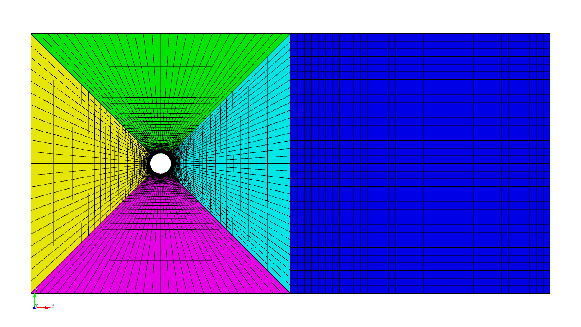
Mesh for a flow past a circular cylinder.
Working with pre_exodus and 4C
pre_exodus is a C++ code embedded into the 4C environment. It is meant to transfer a given mesh into a 4C-readable input file.
Preliminaries
If not already done, compile pre_exodus in the build-release
folder via
make pre_exodus
after configuring 4C in the usual way.
General Procedure of Creating a Valid 4C Input File
With a given mesh including some nodal clouds to apply conditions to you need another text-file (bc-file *) where you specify, what you would like to do with it. It contains for example the specific element declaration (fluid, structure, parameters, etc.) and the particular boundary condition such as Dirichlet or Neumann. Finally, a *header-file consists of general parameters such as solvers, algorithmic parameters, etc. Those three files are merged by pre_exodus into an input file for 4C. This file is then automatically validated using all available 4C validation and is therefore likely to run.
Sure, you usually do not have already a proper header-file and matching bc-file. By typing
./pre_exodus –exo=yourmesh.e
in the build-release folder you get two preliminary files
’default.head’ and ’default.bc’. The first contains the currently valid
header parameters with default values and commented options which you
can edit to adapt it to your means. Similarly, ’default.bc’ consists of
all your mesh entities and a list of all currently valid conditions. See
next section for details how to work with them and how to create valid
input files.
Adapting the header-file
Open the previously created header-file ’default.head’ and edit the following entries as shown below.
PROBLEM TYPEPROBLEMTYPE FluidFLUID DYNAMICLINEAR_SOLVER 1NUMSTEP 20TIMESTEP 0.01SOLVER 1NAME Fluid solverSOLVER UMFPACKMATERIALSinsert the following line in the section
MATERIALSin order to define your material parameters:MAT 1 MAT_fluid DYNVISCOSITY 0.004 DENSITY 1.0FUNCT1insert the following line in the sectionFUNCT1in order to define a time curve:SYMBOLIC_FUNCTION_OF_SPACE_TIME 0.5*(sin((t*pi/0.1)-(pi/2)))+0.5
Save the file under a different name of your choice.
Adapting the bc-file
Open the previously created bc-file ’default.bc’ and edit your boundary conditions as shown below.
----------- Mesh contents -----------

Mesh consists of 7211 Nodes, 7058 Elements, organized in
1 ElementBlocks, 5 NodeSets, 0 SideSets

---------- Syntax examples ----------

Element Block, named:
of Shape: TET4
has 9417816 Elements
'*eb0="ELEMENT"'
sectionname="FLUID"
description="MAT 1 NA Euler"
elementname="FLUID"

Element Block, named:
of Shape: HEX8
has 9417816 Elements
'*eb0="ELEMENT"'
sectionname="STRUCTURE"
description="MAT 1 TECH eas_mild KINEM nonlinear"
elementname="SOLID"

Node Set, named:
Property Name: INFLOW
has 45107 Nodes
'*ns0="CONDITION"'
sectionname="DESIGN SURF DIRICH CONDITIONS"
description="1 1 1 0 0 0 2.0 0.0 0.0 0.0 0.0 0.0  1 none none none none none  1 0 0 0 0 0"

MIND that you can specify a condition also on an ElementBlock, just replace 'ELEMENT' with 'CONDITION'
The 'E num' in the dat-file depends on the order of the specification below
------------------------------------------------BCSPECS

Element Block, named:
of Shape: SHELL4
has 7058 Elements
*eb1="ELEMENT"
sectionname="FLUID"
description="MAT 1 NA Euler"
elementname="FLUID"

Node Set, named: inflow
Property Name: none
has 23 Nodes
*ns1="CONDITION"
sectionname="DESIGN LINE DIRICH CONDITIONS"
description="NUMDOF 3 ONOFF 1 1 0 VAL 1.0 0.0 0.0 FUNCT 1 0 0"

Node Set, named: top
Property Name: none
has 68 Nodes
*ns2="CONDITION"
sectionname="DESIGN LINE DIRICH CONDITIONS"
description="NUMDOF 3 ONOFF 0 1 0 VAL 0.0 0.0 0.0 FUNCT 0 0 0"

Node Set, named: bottom
Property Name: none
has 68 Nodes
*ns3="CONDITION"
sectionname="DESIGN LINE DIRICH CONDITIONS"
description="NUMDOF 3 ONOFF 0 1 0 VAL 0.0 0.0 0.0 FUNCT 0 0 0"

Node Set, named: cylinder
Property Name: none
has 116 Nodes
*ns4="CONDITION"
sectionname="DESIGN LINE DIRICH CONDITIONS"
description="NUMDOF 3 ONOFF 1 1 0 VAL 0.0 0.0 0.0 FUNCT 0 0 0"

Node Set, named: edges
Property Name: none
has 2 Nodes
*ns5="CONDITION"
sectionname="DESIGN POINT DIRICH CONDITIONS"
description="NUMDOF 3 ONOFF 1 1 0 VAL 1.0 0.0 0.0 FUNCT 0 0 0"

-----------------------------------------VALIDCONDITIONS

... remaining stuff has been removed
Save the file under a different name of your choice.
Creating a 4C input file with pre_exodus
The previously created files have to be merged to a 4C input file in
order to solve the problem. We will use pre_exodus for this purpose.
Open a terminal and execute the following command in the
build-release folder:
./pre_exodus --exo=<meshpath>/yourmesh.e --head=<headpath>/headerfile.head
--bc=<bcpath>/bcfile.bc --dat=<datpath>/datfile.dat
Where the filenames and their paths have to be replaced according to how you have named and where you have saved them. pre_exodus will output a dat-file to the path you specified above.
Running a Simulation with 4C
To start the solver use the call
./4C <inputdirectory>/datfile.dat <outputdirectory>/outputprefix
in the build-release folder. You may have to adapt the name of the
executable in this command. The prefix that you have chosen before will
be applied to all output files that 4C generates.
Postprocessing
You can postprocess your results with any visualization software you like. In this tutorial, we choose Paraview.
Filtering result data
Before you can admire your results, you have to generate a filter which converts the generic binary 4C output to the desired format. Starting from the
build-releasedirectory, executemake post_drt_ensight.The filter should now be available in the
build-releasefolder. Filter your results with the following call inside thebuild-releasefolder:./post_drt_ensight - -file=<outputdirectory>/outputprefixFurther options of the filter program are made visible by the command
./post_drt_ensight –help
Visualize your results in Paraview
After the filtering process is finished open paraview by typing
paraview &
File :math:`to` Open and select the filtered
*\*.case*file: outputprefix_fluid.caseChoose LittleEndian instead of BigEndian in case you have an old version of Paraview.
Press Apply to activate the display.
Set the time step in the top menu bar to \(19\) (\(=0.2\)).
In the Color section you can now choose between pressure and velocity. Select velocity and pick the \(X\)-component from the adjacent drop-down menu. Then press the Rescale button and the Show button. You receive a visualization of the \(X\)-velocity field, which should look similar to this figure:
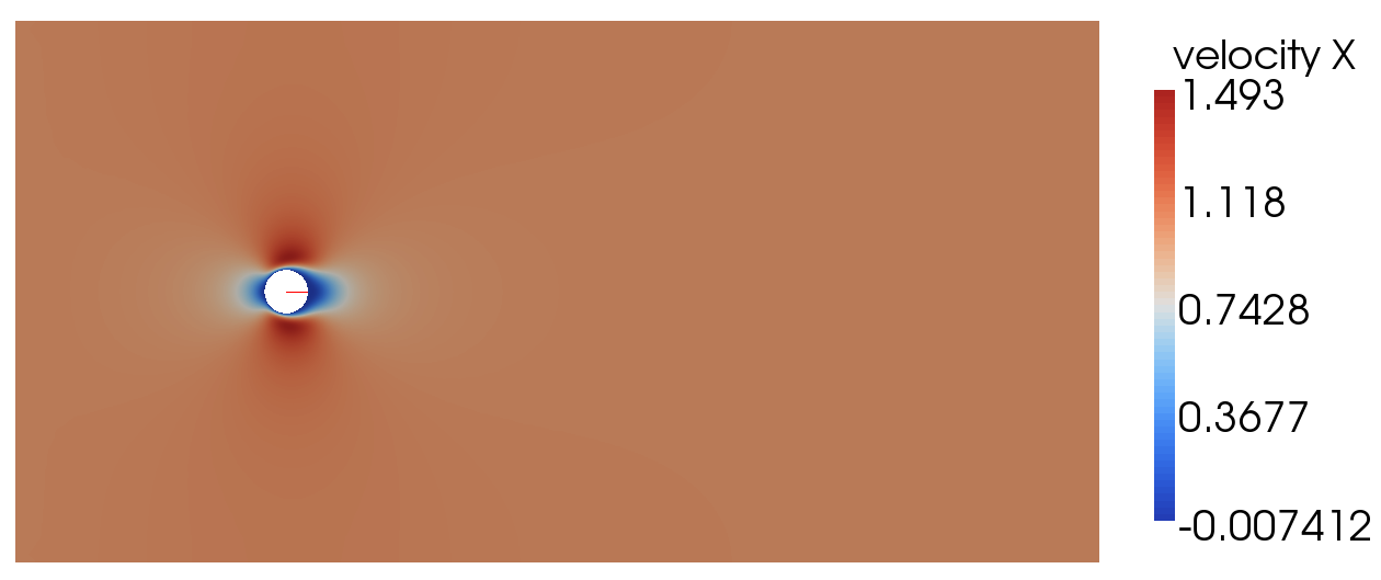
\(X\)-velocity for a flow past a circular cylinder