Solving nonlinear systems in structural simulations
Life is nonlinear, and so are most of the simulations. Thus, the simulation software must be able to deal with nonlinear simulations, be the reason for the nonlinearity a large strain formulation, a nonlinear material model or nonlinear boundary/contact condition.
Since the theory of nonlinear finite element simulations is complex, we will only give an introduction of the necessary input parameters here.
The basic details of the nonlinear solver are given in the section
----------------------STRUCTURAL DYNAMICS
First of all: since in contrast to a linear simulation, where we may scale results (displacements, strains, stresses) with a factor, and also superpose load cases by simply adding results of each load case, the load history is crucial in nonlinear simulations, and we commonly divide the simulation in steps (other programs denote these as increments).
Users may give the time step size, the maximum time at the end of the simulation, and the maximum number of steps to be conducted by these parameters (the values behind the keywords show the default values):
TIMESTEP  0.05
MAXTIME   5
NUMSTEP   200
Note that the simulation stops after NUMSTEP steps or at time=MAXTIME, whatever comes first.
The main decision in a simulation is whether to account for inertia and other time dependent effects, that is, conducting a dynamic simulation, or ignoring these effects and conducting a static simulation. Several options exist for dynamic simulations, while there is only a single option for statics. For the concrete input, see in DYNAMICTYPE.
Time stepping in dynamic simulations
The time stepping in dynamic simulations may be implicit or explicit. While an implicit method involves an iterative procedure within each time step, the explicit solver is solely using the results of the previous time step to calculate the results of the current step. The time stepping procedure is given by the parameter
Explicit time stepping procedure
While it sounds much easier (and thus faster) to base the solution of the current time step on the previous step without iteration, the main drawback is that the time step must be in general much smaller than for an implicit solver. In order to get a correct solution, the time step in an explicit procedure must be small enough that a stress wave cannot travel farther than the smallest element characteristic length in a single time-step. This is called the Courant-Friedrichs-Lewy (CFL) condition. One may calculate this maximum time step size by
Here, \(h\) is the characteristic length of a finite element, \(E, c, \rho\) are the Young’s modulus, the speed of sound and the density of the material, and \(f\) is a safety factor, usually equal to or smaller than 1.
Note
It is the responsibility of the user to choose the time step small enough to get a realistic result in an explicit analysis.
Implicit time stepping procedure
For implicit analyses, a number of time stepping methods exist, the most common of which are
GenAlpha: generalized alpha method with up to four parameters, \(\beta, \alpha_M, \alpha_F, \rho_\infty\), see the reference section –Structural dynamic/GenAlphaOneStepTheta: one-step theta method (a special version of generalized alpha with \(\alpha_M=\alpha_F=1\), see section –Structural dynamic/OneStepTheta
More in-depth information about some time stepping details are given in the theory section below.
Iterative solution
Note that an implicit time stepping procedure involves an iterative solution technique within each time step.
The number of iterations is given in the parameter MAXITER (default: 50); the converge criteria can be defined in a very detailed way with quite a number of parameters.
The strategy for the iteration is specified by the parameter NLNSOL (nonlinear solution). The default is a full Newton-Raphson method, but several other methods exist as well:
Modified Newton-Raphson
Pseudo-transient continuation
Newton-Raphson with line search
linearized Uzawa Iteration within a full Newton-Raphson iteration
NOX Solver, (also includes full Newton with line search)
Warning
Not all methods are available for all simulation cases; e.g., the modified Newton-Raphson can only be used in a multiscale analysis.
The Uzawa Iteration has a number of additional parameters that can be used to improve convergence for special cases.
The convergence can be improved in a dynamic simulation with an aritificial damping (DAMPING) of Rayleigh type or with a material based damping on element-level. If a Rayleigh damping is used, two parameters vary the effect of the damping:
M_DAMPRayleigh-coefficient for Rayleigh damping proportional to mass matrix (\(M_\text{DAMP} \times M\))K_DAMPRayleigh-coefficient for Rayleigh damping proportional to initial/reference stiffness matrix (\(K_\text{DAMP} \times K\))
Convergence difficulties
If the solution does not converge within MAXITER iterations,
one can define the behavior for the step with the parameter DIVERCONT:
stop: stop the simulationcontinue: Simply ignore the missing convergence and continuerepeat_step: Repeat the step (I don’t know the benefit of doing a failed simulation again)halve_step: Reduce the step size of the current increment by 50%.adapt_step: As halve_step reducing the step size by 50%, but checking against the maximum number of cutbacks, which can be given inMAXDIVCONREFINEMENTLEVEL(default: 10). Also the step size may increase by 2 if convergence is achieved four times successively.rand_adapt_step: Changing the time step size by a factor between 0.51 and 1.99, chosen by random number generator. Step size change is alternating between values larger and smaller than 1.0 in consecutive time steps.repeat_simulation: (what the name says - I don’t know what it’s good for…)adapat_penaltycontact: (is not yet implemented for the new time integration scheme)
Theory
Order of accuracy
The difference of an exact solution compared to an approximate solution is called global error \(\boldsymbol{g}\) (Hairer et al. [strdyn:hairer87], Deuflhard et al. [strdyn:deuflhard94]). The global error at time \(t_{n+1}\) can be written as
Although techniques exist to estimate the global error (Hairer et al. [strdyn:hairer87], [strdyn:hairer91]), it is easier to deal with the local discretisation error (cf. Hairer et al. [strdyn:hairer87], Deuflhard et al. [strdyn:deuflhard94]; it is abbreviated with LDE). The global error can be split in a local part and a propagation part. The local part or the local discretisation error, \(\boldsymbol{l}\), contains the error produced in the last integration step \(t_n \to t_{n+1}\). The propagation part, \(\bar{\boldsymbol{g}}\), describes the errors accumulated previous steps. As a consequence, the global error coincides with the local discretisation error for the very first integration step \(\boldsymbol{g}_1 = \boldsymbol{l}_1\), because of the shared initial conditions \(\boldsymbol{y}(t_0) = \boldsymbol{y}_0\)
The term \(\boldsymbol{\Psi}_{n+1,n} \boldsymbol{y}(t_n)\) can be understood as the time integration method but applied to exact rather than approximate values. A Taylor expansion of the local discretisation error leads to an expression in \(\Delta t_n^{p+1}\), where \(p\) is the order of accuracy of the scheme:
The vector function \(\boldsymbol{c}(t_n)\) depends on the time integration scheme. In the case of Runge-Kutta methods \(\boldsymbol{c}\) has the form \(\boldsymbol{c}(t_n) = K \frac{\mathrm{d}^{p+1} \boldsymbol{y}(t_n)}{\mathrm{d} t^{p+1}}\) with a constant \(K \neq 0\).
If the approximate solution converges to the exact solution for \(\Delta t_n\to0\), the scheme is called consistent. Consistency requires \(p\geq1\). This is because the global error is \(\mathcal{O}(\Delta t_n^p)\). The reduced power of the global error stems from the propagation of the local errors in time.
Generalised-alpha time-stepping procedure
Newmark’s method
Newmark’s method is a family of schemes with two parameters \(\gamma\in[0,1]\) and \(\beta\in[0,\frac{1}{2}]\). The basic assumption of Newmark’s method is a linear approximation of the acceleration \(\boldsymbol{A}\) within the time step.
The integration parameter \(\tau\) is defined on the interval \([t_n,t_n+1]\) as \(\tau \in[0,\Delta t]\). Now, two parameters are introduced to control the behavior of this approximation
If \(\gamma=\frac{1}{2}\) and \(\beta=\frac{1}{6}\) are chosen, a linear acceleration scheme is obtained. The \(\gamma\)-parameterized acceleration \(\boldsymbol{A}^\gamma(\tau)\) is integrated once over \(\tau\), which yields
The integration constant \(c\) is defined by inserting the known boundary condition of the integral \(\boldsymbol{V}(\tau=0) = \boldsymbol{V}_n\), which gives
The new timesteps velocity \(\boldsymbol{V}_{n+1}\) is therefore obtained at \(\boldsymbol{V}(\tau = \Delta t)\)
Likewise, the \(\beta\)-parameterized acceleration \(\boldsymbol{A}^\beta(\tau)\) is integrated to obtain the velocity
To obtain the displacement approximation, we integrate again over \(\tau\) and yield
Inserting the boundary condition \(\boldsymbol{D}(\tau=0) = \boldsymbol{D}_n\), we get the displacement \(\boldsymbol{D}_{n+1} = \boldsymbol{D}(\tau = \Delta t)\) at the end of the time interval:
Now we can express the new time steps velocity and acceleration solely from old time steps values and the new displacement as
The final pair of equations can be rewritten such that (with \(\beta\in[0,\frac{1}{2}]\)):
with \(\beta \in [0,\frac{1}{2}], \, \gamma \in [0,1]\).
Here, we abbreviated the unknown accelerations at \(t_{n+1}\) with \(\boldsymbol{A}_{n+1} = \boldsymbol{M}^{-1} \big( -\boldsymbol{C} \boldsymbol{V}_{n+1} - \boldsymbol{F}_{\text{int};n+1} + \boldsymbol{F}_{\text{ext};n+1}) \big)\).
This temporal discretisation leads to a fully discretised set of equations of motion:
This completely discretised equation of motion is primarily an \(\mathit{ndof}\)-dimensional system of nonlinear equations in the unknown displacements \(\boldsymbol{D}_{n+1}\). This statements can be clarified by writing Newmark’s method such that the velocity and acceleration at \(t_{n+1}\) are given depending on the displacements \(\boldsymbol{D}_{n+1}\):
Generalised-alpha method
The key idea behind the generalised-alpha method [strdyn:chung95] is a modification of the time point at which the discretised equations of motion is evaluated. Newmark’s method searches for equilibrium at the end of the current time step \([t_n,t_{n+1}]\), i.e.at the time \(t_{n+1}\). The generalised-alpha method shifts this evaluation point to generalised mid-points \(t_{n+1-\alpha_\text{f}}\) and \(t_{n+1-\alpha_\text{m}}\), respectively. The non-linear equation of motion becomes at the generalised mid-point
\[\boldsymbol{M} \boldsymbol{A}_{n+1-\alpha_\text{m}} + \boldsymbol{C} \boldsymbol{V}_{n+1-\alpha_\text{f}} + \boldsymbol{F}_{\text{int};n+1-\alpha_\text{f}} = \boldsymbol{F}_{\text{ext};n+1-\alpha_\text{f}}\]
The mid accelerations, velocities, displacements and external forces are defined as linear combinations of the corresponding start and end vector:
with the parameters \(\alpha_\text{m},\alpha_\text{f}\in[0,1]\). There two possibilities for the internal mid-forces \(\boldsymbol{F}_{\text{int},\text{mid}}\). Either they are defined as well by a linear combination (which we call ‘TR-like’) or by inserting mid-displacements (which we call ‘IMR-like’), i.e.
*TR-like
IMR-like
The end-point accelerations and velocities, i.e. \(\boldsymbol{A}_{n+1}\) and \(\boldsymbol{V}_{n+1}\), are related linearly to the end-point displacements \(\boldsymbol{D}_{n+1}\) by Newmark’s method (5). Therefore, the mid-equilibrium can be still thought of a system of nonlinear equations in \(\boldsymbol{D}_{n+1}\). Let us again write the unknown mid-velocities and mid-accelerations in terms of \(\boldsymbol{D}_{n+1}\):
The mid-point internal force vector means in terms of assembled element force vectors:
text{TR-like}
IMR-like
Linearisation and Newton–Raphson iteration
The generalised mid-point-discretised linear momentum balance can be written as an residual
\[\boldsymbol{R}_\text{effdyn}(\boldsymbol{D}_{n+1}) = \boldsymbol{M} \boldsymbol{A}_{n+1-\alpha_\text{m}} + \boldsymbol{C} \boldsymbol{V}_{n+1-\alpha_\text{f}} + \boldsymbol{F}_{\text{int};n+1-\alpha_\text{f}} - \boldsymbol{F}_{\text{ext};n+1-\alpha_\text{f}} \stackrel{!}{=} \boldsymbol{0}\]These nonlinear equations can be linearised at the end of the time step at \(t_{n+1}\) with \(\boldsymbol{D}_{n+1}\):
\[Lin\boldsymbol{R}_\text{effdyn}(\boldsymbol{D}_{n+1}) = \boldsymbol{R}_\text{effdyn}(\boldsymbol{D}_{n+1}^i) + \left.\frac{\partial\boldsymbol{R}_\text{effdyn}(\boldsymbol{D}_{n+1})} {\partial\boldsymbol{D}_{n+1}}\right|^{i} \Delta\boldsymbol{D}_{n+1}^{i+1}\]
in which the dynamic effective tangential stiffness matrix \(\boldsymbol{K}_{\text{T}\,\text{effdyn}}\) appears as the differentiation of the dynamic effective residual with respect to the displacements \(\boldsymbol{D}_{n+1}\). This stiffness matrix is obtained detailed in
with
In a Newton–Raphson iteration the iterative displacement increment \(\Delta\boldsymbol{D}_{n+1}^{i+1}\) is calculated by solving
This allows to update the unknown displacements with
In essence, the actual right-hand-side \(\boldsymbol{R}_\text{effdyn}(\boldsymbol{D}_{n+1}^{i})\) depends as shown only on the actual end-displacements \(\boldsymbol{D}_{n+1}^{i+1}\), but it is convenient to calculate \(\boldsymbol{R}_\text{effdyn}(\boldsymbol{D}_{n+1}^i)\) using the current mid-displacements, -velocities and -accelerations. These current vectors can be calculated based on the formulas given in (6) or (7). Optionally, they can be evaluated with an update mechanism with these increments
and the usual update procedure
The convergence of the Newton–Raphson iteration can be tested — for instance — by checking the residual
A different relative convergence check is based on the displacement increment:
Algorithm Newton–Raphson iteration
Note
struktogramm to be added.
Here we have used a very simple predictor for the new displacements (and in consequence for velocities and accelerations): The previously converged time step is used. More sophisticated predictors can be constructed introducing extrapolation techniques or explicit time integration schemes. For instance, the forward Euler time integration scheme could be applied as a predictor (forward Euler was introduced in the course “Finite Elemente”); however, forward Euler is not a recommended choice.
Order of accuracy
According to the consideratins above, we can deduce the order of accuracy of the displacement approximation given by the generalised-alpha (GA) method. We achieve
This equation implies: The displacements are always at least second order accurate and they are even third order accurate if \(\frac{1}{3} - 2\beta + \alpha_\text{f} - \alpha_\text{m} = 0\).
Since the governing equations are a set of second order ODEs, we provide the LDE of the velocities as well. These are
in which \(\dot{\boldsymbol{l}}_{n+1}^{\text{GA}}\) and \(\dot{\boldsymbol{\Psi}}_{n+1,n}^{\text{GA}}\) do not imply a time differentation – the dot is merely a notation. It can be seen the velocities are second order accurate if \(\frac{1}{2} - \gamma + \alpha_\text{f} - \alpha_\text{m}\) otherwise only first order.
The order of accuracy of the generalised-alpha method follows the lower value of the order of the displacements or velocities.
As stated before, the semi-discrete equations of motion are second order ODE, thus both LDEs have to be taken into account and the worse value determines the overall order of accuracy according to Hairer et al [strdyn:hairer87], [strdyn:hairer91])
Time adaptivity
This section is an excerpt of [strdyn:bornemann03].
Based on indication of the local discretisation error
Different ways exist to adapt the time step size \(\Delta t\), here we only apply an a posteriori method utilising the local discretisation error (LDE).
Step size adaptivity
Local error control is based on requiring the estimated local discretisation error to stay below a user-defined tolerance \(\mathit{tol}\). If the local discretisation error, resulting from a time integration with time step size \(\Delta t_n\), is higher than the tolerance, the step is repeated with a smaller step size. A proposal for this smaller step size is the so-called ‘optimal’ step size, denoted with \(\Delta t_n^*\), which is the time step size resulting in a local discretisation error which is approximately equal to the tolerance. The procedure is repeated until a small enough step size is found. Then the ‘optimal’ time step size might be used as an initial value for the next time step size \(\Delta t_{n+1} = \Delta t_n^*\).
Therefore the basic requirement for the local discretisation error is
whereby the dimensionless tolerance \(\varepsilon>\) is user-prescribed. The above described procedure is contained in the following figure:
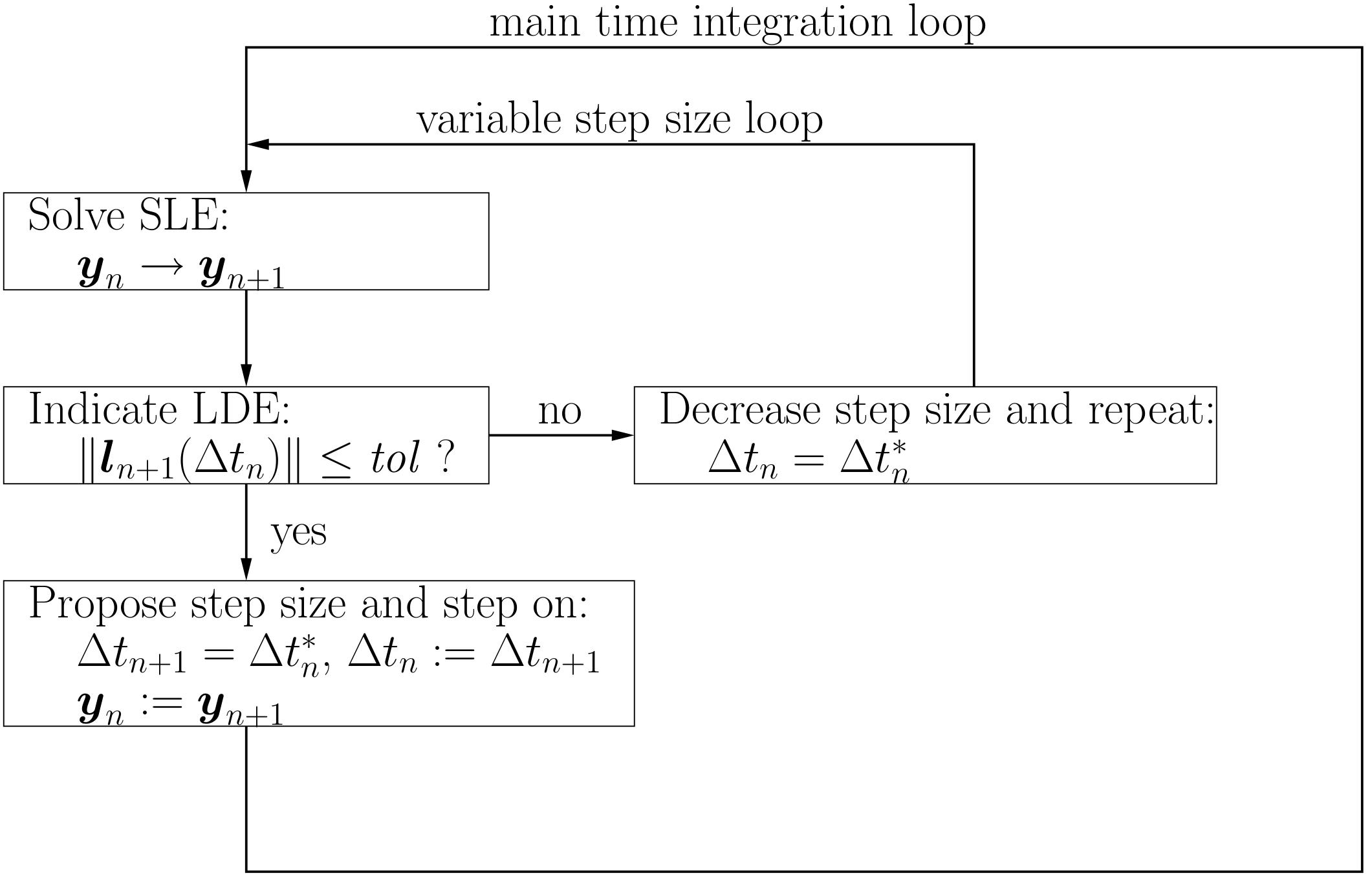
Diagram of LDE-based step size adaptivity
Different norms, such as average, root-mean-square or infinity norm, can be used to obtain a dimensionless scalar from the local discretisation error vector.
The ‘optimal’ step size \(\Delta t_n^*\) is derived in the following equations. The starting point is the usual definition of the local discretisation error in which the local discretisation error obtained with \(\Delta t_n\) is assumed to be larger than \(\mathit{tol}\):
The second equation can be transformed to
Introducing this equation into the first one from above, we get
The ‘optimal’ step size corresponds to the lower bound in this equation.
Furthermore, the ‘optimal’ step size might be more reliable if the tolerance is reduced by ‘safety’ scale factors
In the previous equation the ‘optimal’ ratio is abbreviated with
The step size \(\Delta t_n^\text{new}\), see above, replaces the ‘optimal’ step size \(\Delta t_n^*\) in the outlined algorithm. The factor \(r_\text{max}\) limits the maximum size increase between two steps, \(r_\text{min}\) bounds the decrease. In the same spirit, a maximum and minimum step size, \(\Delta t_\text{max}\) and \(\Delta t_\text{min}\), is imposed to achieve a more robust algorithm. Sometimes, \(p\) instead of \((p+1)\) is used in the equation for \(r ^*\) to reflect the order of the global error.
Generally speaking, estimations for the local discretisation error are obtained by using two different time integration schemes A and B. The comparison of results \(\boldsymbol{y}_{n+1}^\text{A}\) to \(\boldsymbol{y}_{n+1}^\text{B}\) makes it possible to evaluate an local discretisation error estimation of the lower-order method of scheme A or B. If the results of the scheme A are kept to integrate forward in time, then A is called marching time integration scheme. The scheme B is only used to indicate the local discretisation error, hence it is referred to as auxiliary scheme. The adaptive algorithm is denoted with B/A.
The algorithms based on embedded Runge-Kutta methods are instances of such local error control with time step adaption.
Zienkiewicz and Xie indicator
Zienkiewicz and Xie presented in [strdyn:zienkiewicz91] a local error indicator for the Newmark algorithm. The estimator advantageously uses the member which integrates the displacements with third-order accuracy, i.e., \(\beta=\frac{1}{6}\), \(\gamma\) arbitrary. The concept can be straight forwardly applied to the generalised-alpha method.
In essence, the general generalised-alpha method with second order accurate displacements (dubbed here GA2) is considered as the marching time integration scheme. Its third order accurate sibling GA3 is used as the auxiliary scheme to eventually obtain the local discretisation error estimation/indication of the displacements.
The GA2 and GA3 methods are implicit schemes, hence a direct calculation with GA2 and GA3 would require two iterative solutions. This can be overcome by avoiding a direct determination of the GA3. The results of the marching GA2 method (\(\boldsymbol{D}_{n+1}^\text{GA2}\), \(\boldsymbol{V}_{n+1}^\text{GA2}\), \(\boldsymbol{A}_{n+1}^\text{GA2}\)) can be used to explicitly construct a third-order accurate result, which is related to the NM3 and is called ZX here.
The ZX method is defined as
The dependence of this algorithm on \(\boldsymbol{D}_{n+1}^\text{GA2}\) is revealed by introducing (13)
The local discretisation error of the ZX is based on (13) by expanding it in Taylor series:
in which the third-order accuracy is shown.
Zienkiewicz and Xie’s indicator of the local discretisation error uses the definitions of the local discretisation errors for the displacements and assumes direct differences as feasible approximations
The above equations (14) are subtracted from each other leading to
as \(\boldsymbol{l}_{n+1}^\text{ZX}\) is negligible compared to \(\boldsymbol{l}_{n+1}^\text{GA2}\). The indicator is given alternatively as
which coincides with the formula of Zienkiewicz and Xie [strdyn:zienkiewicz91] except the sign.
The presented local discretization error estimator allows only to assess the displacements, the velocities are not checked.