Debugging and Profiling Tools

In software development sooner or later one experiences that written software does not always behave as intended, or with the performance as expected. This is were debugging and profiling tools come to hand that help understand what software is actually doing, or identify bottlenecks in the program execution. However, not only software developers, also users of software written by others may benefit from debugging and profiling tools.

Overview of debugging and profiling tools

In the following various debugging and profiling tools are described that may be of help when developing or working with 4C.

Get MPI collective timer statistics with a time monitor from Trilinos package Teuchos
Code profiling of 4C with callgrind
Debugging/MPI debugging with VS Code

Useful options for Debugging with gdb (or your IDE)

Build debug version

Create a directory, where you want to build your debug version and build a 4C with debug flag using the correct preset. This should contain:

{
  "name": "debug",
  "displayName": "Debug build for a general workstation",
  "binaryDir": "<4C-debug-execdir>",
  "generator": "Ninja",
  "inherits": [
    "lnm_workstation"
  ],
  "cacheVariables": {
    "CMAKE_BUILD_TYPE": "DEBUG"
  }
}

Pretty printing of the Standard Library

Add the following to your ~/.gdbinit

python
import sys
sys.path.insert(0, '/usr/share/gcc/python')
from libstdcxx.v6.printers import register_libstdcxx_printers
register_libstdcxx_printers (None)
end

enable pretty-printer

Useful settings for MPI Debugging

“Standard” parallel errors

In this mode, all processes are paused once one process hits a debug event:

set detach-on-fork off
set schedule-multiple on

Tracking down race conditions

If you have to track down race conditions, you need manual control over each process. You can start attach gdb to each process after it has already started. Start 4C via

mpirun -np 2 ./4C ../path/to/input.dat ../path/to/output --interactive

The process id of each mpi process is being displayed. Once all gdb instances are connected, you can press any key to start the execution.

gdb + valgrind to track down memory leaks / invalid reads/writes

valgrind --tool=memcheck -q --vgdb-error=0 ./4C path/to/input.dat path/to/output

Then, you can connect with a gdb debugger:

gdb ./4C
(gdb) target remote | bgdb --pid=<insert pid here>

Or visually using VS Code:

Add a configuration in launch.json:

{
  "name": "(gdb) Attach to valgrind",
  "type": "cppdbg",
  "request": "launch",
  "program": "<4C-debug-execdir>",
  "targetArchitecture": "x64",
  "customLaunchSetupCommands": [
    {
      "description": "Enable pretty-printing for gdb",
      "text": "-enable-pretty-printing",
      "ignoreFailures": true
    },
    {
      "description": "Attach to valgrind",
      "text": "target remote | vgdb --pid=<insert pid here>",
      "ignoreFailures": false
    }
  ],
  "stopAtEntry": false,
  "cwd": "/path/to/run/",
  "environment": [],
  "externalConsole": false,
  "MIMode": "gdb"
}

If you need to run it in combination with mpirun, start it with

mpirun -np 2 valgrind --tool=memcheck -q --vgdb-error=0 ./4C path/to/input.dat path/to/output

and connect to each process individually.

Code profiling with `callgrind`

“Callgrind is a profiling tool that records the call history among functions in a program’s run as a call-graph. By default, the collected data consists of the number of instructions executed, their relationship to source lines, the caller/callee relationship between functions, and the numbers of such calls.” (from callgrind)

Configure and build for profiling

Note: For general information about configuring and building of 4C refer to Configure and Build and the README.md.

You probably want to configure with CMAKE_BUILD_TYPE set to RELWITHDEBINFO. This results in a release version of the 4C build with additional per-line annotations. That way, when examining the results one can see the exact lines of code where computation time is spent.

Note

Beware that code gets inlined with the profiling build of 4C and hot spots might appear within the inlined section.
The debug version of 4C also contains per-line annotations but without the effect of inlining and can thus also be used to profile 4C. However, the debug version is compiled without compiler optimizations and thus does not give a representative view of hot spots.
For a quick profiling without per-line annotations also the release version can be used. This already gives a nice overview of computationally expensive methods.

Run simulation with valgrind

Run a 4C simulation with valgrind in parallel using the command:

mpirun -np <numProcs> valgrind --tool=callgrind <someBaseDir>/<4C-execdir>/4C <inputfile> <output>

In addition to the usual 4C output, valgrind writes output for each mpi rank in the files callgrind.out.<processId>.

Note

For profiling a simulation in serial execute:

valgrind --tool=callgrind <someBaseDir>/<4C-execdir>/4C <inputfile> <output>

It is also possible to examine the post processing of result files, simply wrap the corresponding command:
```
mpirun -np <numProcs> valgrind --tool=callgrind <command>
```
Wrapping the 4C simulation using valgrind increases the runtime by a factor of about 100. Therefore, to reduce the total wall time think about running only a few time steps of your 4C simulation. Depending on the problem type it might be reasonable to do this after a restart in order to examine characteristic parts. Follow the steps as described below:
```
mpirun -np <numProcs> <someBaseDir>/<4C-execdir>/4C <inputfile> <output>
mpirun -np <numProcs> valgrind --tool=callgrind <someBaseDir>/<4C-execdir>/4C <inputfile> <output> restart=<restartStep>
```

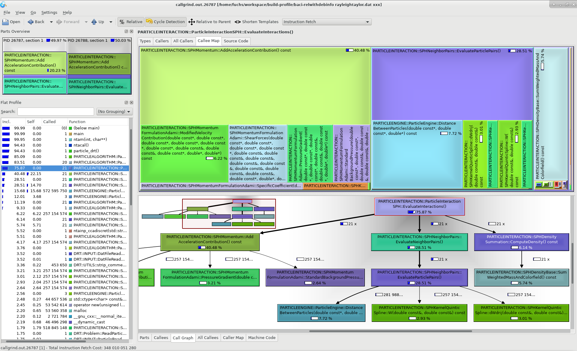
Examine results with `kcachegrind`

Using kcachegrind (refer to kcachegrind for documentation and download) the output can be visualized via:

kcachegrind callgrind.out.*

It is also possible to only open the output of a specific mpi rank with processor id <processId> via:

kcachegrind callgrind.out.<processId>

Note: Be sure to check out the 4C version the code is compiled with in your local git repo to make use of the per-line annotations.

Example: In the figure below a screenshot of kcachegrind is given where the profiling output of a Smoothed Particle Hydrodynamics (SPH) simulation is visualized.

Teuchos Time Monitor

The TimeMonitor from Trilinos package Teuchos provides MPI collective timer statistics. Refer to the Teuchos::TimeMonitor Class Reference https://trilinos.org/docs/dev/packages/teuchos/doc/html/classTeuchos_1_1TimeMonitor.html for a detailed documentation.

Add a timer for a method in 4C

In order to get parallel timing statistics of a method in 4C include the following header

#include <Teuchos_TimeMonitor.hpp>

in the .cpp-file that contains the implementation of the method and add the macro TEUCHOS_FUNC_TIME_MONITOR with the name of the method in the implementation of the method:

void <NAMESPACE>::<FunctionName>(...)
{
  TEUCHOS_FUNC_TIME_MONITOR("<NAMESPACE>::<FunctionName>");

  /* implementation */
}

Running a simulation on 3 processors for example yields the following TimeMonitor output in the terminal:

============================================================================================================

                                   TimeMonitor results over 3 processors

Timer Name                   MinOverProcs       MeanOverProcs      MaxOverProcs       MeanOverCallCounts
------------------------------------------------------------------------------------------------------------
<NAMESPACE>::<FunctionName>  0.1282 (1000)      0.2134 (1000)      0.2562 (1000)      0.0002132 (1001)
============================================================================================================

The output gives the minimum, maximum, and mean execution time (number of counts) for all processors and also the mean execution time over all counts.

Note: The TimeMonitor output of a 4C simulation in general already contains a variety of methods that are monitored, meaning there is a line with timings for each method in the output.

How to interpret the output of the `TimeMonitor`

Examining the output of the TimeMonitor is probably one of the easiest steps in profiling the behaviour of a program. The information given in the output of the TimeMonitor may server for

getting an idea of the execution time of a method
knowing how often a method is called during the runtime of the program
investigating the parallel load balancing of a method (compare MinOverProcs with MaxOverProcs)

and thereby helps identifying bottlenecks in the overall program.