FSI Tutorial 3D
Introduction
As example, we consider a 3d driven cavity example as sketched in the figure below with a depth of 0.05. For further details and references we refer the reader to [Wall99].
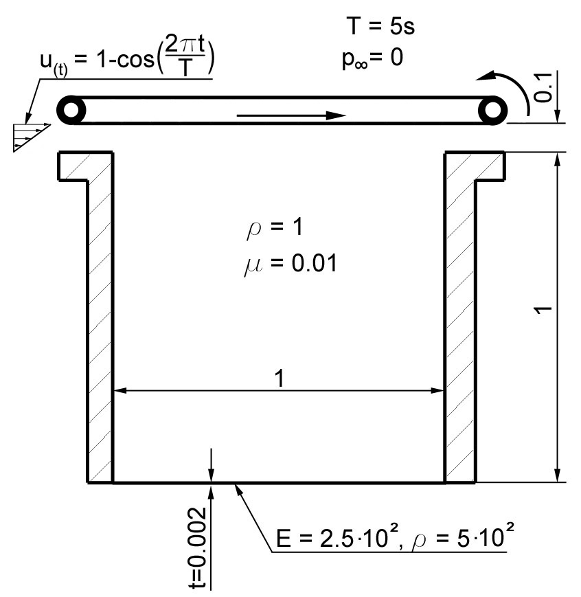
The driven cavity example
Creating the Geometry with Cubit
Besides meshing cubit also has several geometry creation methods. We refer to the provided manual and tutorials. It supports scripting (also Python), therefore we provide the following Journal-file containing the necessary geometry commands as well as mesh and definitions for elements and boundary conditions, respectively.
You can find the complete journal in tests/tutorials/tutorial_fsi_3d.jou.
Within Cubit, run the journal file (Tools \(\to\) Play journal file \(\to\) open the journal file mentioned above). Export the created geometry and mesh to an EXODUS file of your choice via File \(\to\) Export…. During export, set the dimension explicitly to 3D.
Creating the 4C input file
Geometry description
The geometry is described in the file tutorial_fsi_3d.e we created before. It contains two element blocks for the fluid and the structure domain, respectively. We reference this file in the input file and assign the correct element types and material properties to the blocks:
STRUCTURE GEOMETRY:
  FILE: tutorial_fsi_3d.e
  SHOW_INFO: summary
  ELEMENT_BLOCKS:
  - ID: 1
    SOLID:
      HEX8:
        MAT: 1
        KINEM: nonlinear
        TECH: eas_full
FLUID GEOMETRY:
  FILE: tutorial_fsi_3d.e
  ELEMENT_BLOCKS:
  - ID: 2
    FLUID:
      HEX8:
        MAT: 2
        NA: ALE
MATERIALS:
- MAT: 1
  MAT_Struct_StVenantKirchhoff:
    YOUNG: 1000
    NUE: 0.3
    DENS: 500
- MAT: 2
  MAT_fluid:
    DYNVISCOSITY: 0.01
    DENSITY: 1
- MAT: 3
  MAT_Struct_StVenantKirchhoff:
    YOUNG: 500
    NUE: 0.3
    DENS: 500
General parameters
Since we want to run a fluid-structure interaction simulation, we need to set the parameters for the fluid, the structure and the ALE subproblems. First, let us specify the type of problem:
PROBLEM TYPE:
  PROBLEMTYPE: Fluid_Structure_Interaction
We set the following parameters for the structure problem:
STRUCTURAL DYNAMIC:
  INT_STRATEGY: Standard
  LINEAR_SOLVER: 3
SOLVER 1:
  SOLVER: UMFPACK
For the fluid problem we set the following parameters:
FLUID DYNAMIC:
  LINEAR_SOLVER: 2
  ADAPTCONV: true
SOLVER 2:
  SOLVER: Belos
  NAME: Fluid solver
For the ALE problem, we set the following parameters:
ALE DYNAMIC:
  LINEAR_SOLVER: 1
FSI DYNAMIC:
  NUMSTEP: 3
A couple of different conditions are applied:
Surface clamping conditions and fixtures are left out here for the sake of brevity. Refer to the complete input file for details.
The prescribed velocity at the top of the cavity is defined via a function:
FUNCT1:
- SYMBOLIC_FUNCTION_OF_SPACE_TIME: (1-cos(2*t*pi/5))
The coupling surface between fluid and structure domain is specified as
DESIGN FSI COUPLING SURF CONDITIONS:
- E: 5
  ENTITY_TYPE: node_set_id
  coupling_id: 1
- E: 14
  ENTITY_TYPE: node_set_id
  coupling_id: 1
Running the simulation
Run the simulation by providing the created input and an output prefix to 4C and postprocess the results.
Postprocessing
You can postprocess your results with any visualization software you like. In this tutorial, we choose Paraview.
Before you can open the results, you have to generate a filter again. Call make post_ensight in the 4C-directory. Filter your results in the output directory with the call
./post_ensight --file=[outputdirectory]/outputprefix
After this open paraview, go to
File \(\to\) Open Data and select the filtered *.case file.
Only for older versions of Paraview:
Select the time step in the Select Time Value window on the left and
shift Byte order to little endian
Click on accept (or apply) to activate the display.
In the Display tab (section Color) you can choose now between Point pressure and Point velocity, whatever you want to display.
For the scale, activate the Scalar bar button in the View section.