FSI Tutorial 2D
Introduction
We consider a 2d driven cavity example as sketched in Fig. 1.1. For further details and references we refer the reader to [Wall99]
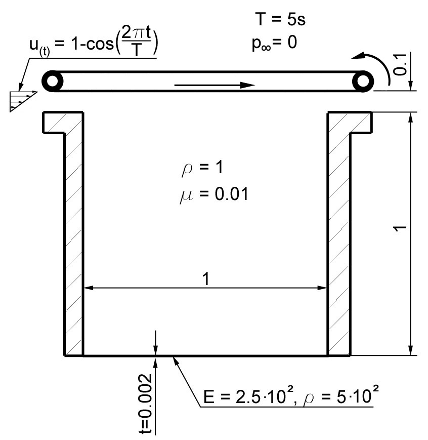
The driven cavity example in 2d
You can find the complete journal in tests/tutorials/tutorial_fsi.jou.
Within Cubit, open the Journal-Editor (Tools\(\to\)Journal Editor), paste the text from the journal file and press play.
Export the created geometry and mesh to an EXODUS file via File\(\to\)Export…. During export, set the dimension explicitly to 2D.
The FSI problem with a partitioned solver
Here, we create the 4C input file for the FSI problem, that is solved using a partitioned scheme, which means that the fluid and the solid problem are solved sequentially. For a monolithic scheme, see the section below.
Geometry description
The geometry is described in the file tutorial_fsi_2d.e we created before. It contains two element blocks for the fluid and the structure domain, respectively. We reference this file in the input file and assign the correct element types and material properties to the blocks:
STRUCTURE GEOMETRY:
  FILE: tutorial_fsi_2d.e
  ELEMENT_BLOCKS:
  - NAME: flexible_bottom
    SOLID:
      QUAD4:
        MAT: 2
        KINEM: nonlinear
        THICKNESS: 1.0
        PLANE_ASSUMPTION: plane_strain
FLUID GEOMETRY:
  FILE: tutorial_fsi_2d.e
  SHOW_INFO: summary
  ELEMENT_BLOCKS:
  - NAME: fluid
    FLUID:
      QUAD4:
        MAT: 1
        NA: ALE
MATERIALS:
- MAT: 1
  MAT_fluid:
    DYNVISCOSITY: 0.01
    DENSITY: 1
- MAT: 2
  MAT_ElastHyper:
    NUMMAT: 1
    MATIDS:
    - 3
    DENS: 500
- MAT: 3
  ELAST_CoupNeoHooke:
    YOUNG: 250
- MAT: 4
  MAT_Struct_StVenantKirchhoff:
    YOUNG: 1
    NUE: 0
    DENS: 1
General parameters
We set the following parameters in the input file:
PROBLEM TYPE:
  PROBLEMTYPE: Fluid_Structure_Interaction
ALE DYNAMIC:
  ALE_TYPE: springs_spatial
  MAXITER: 4
  TOLRES: 0.0001
  TOLDISP: 0.0001
  RESULTSEVERY: 1
  LINEAR_SOLVER: 1
FLUID DYNAMIC:
  LINEAR_SOLVER: 2
  TIMEINTEGR: Np_Gen_Alpha
  GRIDVEL: BDF2
  ADAPTCONV: true
  ITEMAX: 50
STRUCTURAL DYNAMIC:
  INT_STRATEGY: Standard
  M_DAMP: 0.5
  K_DAMP: 0.5
  TOLDISP: 1e-12
  TOLRES: 1e-12
  TOLPRE: 1e-10
  TOLINCO: 1e-10
  PREDICT: ConstDisVelAcc
  LINEAR_SOLVER: 3
FSI DYNAMIC:
  MAXTIME: 3
  NUMSTEP: 3
  SECONDORDER: true
SOLVER 1:
  SOLVER: UMFPACK
  AZSUB: 300
  NAME: ALE solver
SOLVER 2:
  SOLVER: Belos
  AZTOL: 1e-12
  AZSUB: 300
  NAME: Fluid solver
SOLVER 3:
  SOLVER: UMFPACK
  AZSUB: 300
  NAME: Structure solver
We define the domain of the ALE problem as a clone of the fluid domain and assign a material:
CLONING MATERIAL MAP:
- SRC_FIELD: fluid
  SRC_MAT: 1
  TAR_FIELD: ale
  TAR_MAT: 4
FUNCT 1insert
SYMBOLIC_FUNCTION_OF_SPACE_TIME (1-cos(2*t*pi/5))defining time-dependent inflow and lid movementFUNCT 2insert
SYMBOLIC_FUNCTION_OF_SPACE_TIME 10*(y-1)*(1-cos(2*t*pi/5))representing the spatial inflow distribution
Safe the file under a different name, e.g. ’dc2d_fsi.head’.
Boundary conditions
The boundary conditions are set as follows:
Dirichlet boundary conditions for structure, fluid and ALE:
DESIGN LINE DIRICH CONDITIONS:
- NODE_SET_NAME: structure_clamping_curves
  NUMDOF: 2
  ONOFF:
  - 1
  - 1
  VAL:
  - 0
  - 0
  FUNCT:
  - 0
  - 0
- NODE_SET_NAME: cavity_wall_curves
  NUMDOF: 3
  ONOFF:
  - 1
  - 1
  - 0
  VAL:
  - 0
  - 0
  - 0
  FUNCT:
  - 0
  - 0
  - 0
- NODE_SET_NAME: inflow_volume_curve_top
  NUMDOF: 3
  ONOFF:
  - 1
  - 1
  - 0
  VAL:
  - 1
  - 0
  - 0
  FUNCT:
  - 1
  - 0
  - 0
- NODE_SET_NAME: inflow_area_curve
  NUMDOF: 3
  ONOFF:
  - 1
  - 1
  - 0
  VAL:
  - 1
  - 0
  - 0
  FUNCT:
  - 2
  - 0
  - 0
DESIGN POINT DIRICH CONDITIONS:
- NODE_SET_NAME: structure_vertices
  NUMDOF: 2
  ONOFF:
  - 1
  - 1
  VAL:
  - 0
  - 0
  FUNCT:
  - 0
  - 0
- NODE_SET_NAME: structure_fsi_vertices
  NUMDOF: 2
  ONOFF:
  - 1
  - 1
  VAL:
  - 0
  - 0
  FUNCT:
  - 0
  - 0
- NODE_SET_NAME: inflow_vertices_top
  NUMDOF: 3
  ONOFF:
  - 1
  - 1
  - 0
  VAL:
  - 1
  - 0
  - 0
  FUNCT:
  - 1
  - 0
  - 0
- NODE_SET_NAME: cavity_vertices
  NUMDOF: 3
  ONOFF:
  - 1
  - 1
  - 0
  VAL:
  - 0
  - 0
  - 0
  FUNCT:
  - 0
  - 0
  - 0
- NODE_SET_NAME: fluid_fsi_vertices
  NUMDOF: 3
  ONOFF:
  - 1
  - 1
  - 0
  VAL:
  - 0
  - 0
  - 0
  FUNCT:
  - 0
  - 0
  - 0
DESIGN LINE ALE DIRICH CONDITIONS:
- NODE_SET_NAME: inflow_volume_curve_top
  NUMDOF: 2
  ONOFF:
  - 1
  - 1
  VAL:
  - 0
  - 0
  FUNCT:
  - 0
  - 0
- NODE_SET_NAME: fluid_curves_in_y-direction
  NUMDOF: 2
  ONOFF:
  - 1
  - 1
  VAL:
  - 0
  - 0
  FUNCT:
  - 0
  - 0
DESIGN POINT ALE DIRICH CONDITIONS:
- NODE_SET_NAME: fluid_vertices_all
  NUMDOF: 2
  ONOFF:
  - 1
  - 1
  VAL:
  - 0
  - 0
  FUNCT:
  - 0
  - 0
FSI coupling conditions:
DESIGN FSI COUPLING LINE CONDITIONS:
- NODE_SET_NAME: structure_fsi_curve
  coupling_id: 1
- NODE_SET_NAME: fluid_fsi_curve
  coupling_id: 1
Running the Simulation
Run in a shell
./4C <input_file_name> <output_directory>/output_prefix
Postprocessing
Warning
The procedure described here is likely outdated and needs to be update by the output taskforce!
You can postprocess your results with any visualization software you like. In this tutorial, we choose Paraview.
Before you can open the results, you have to generate a filter again. Call make post_ensight in the 4C-directory. Filter your results in the output directory with the call
./post_ensight --file=[outputdirectory]/outputprefix
After this open paraview, go to
File:math:`to`Open Data and select the filtered *.case file.
Only for older versions of Paraview:
Select the time step in the Select Time Value window on the left and
shift Byte order to little endian
Click on accept (or apply) to activate the display.
In the Display tab (section Color) you can choose now between Point pressure and Point velocity, whatever you want to display.
Use a warp vector to visualize the simulation results on the deformed domain.
For the scale, activate the Scalar bar button in the View section.
The FSI problem with a monolithic solver
There are two possibilities for monolithic schemes:
fluid-split: the fluid field is chosen as slave field, the structure field is chosen as master field.
structure-split: the structure field is chosen as slave field, the fluid field is chosen as master field.
In order to use a monolithic solver, change the coupling algorithm
COUPALGO in the FSI DYNAMIC section in the *.head-file.
Additionally, special care has to be taken of the interface degrees of
freedom, that are subject to Dirichlet boundary conditions. The
interface is always governed by the master field. The slave interface
degrees of freedom do not occur in the global system of equations and,
thus, are not allowed to carry Dirichlet boundary conditions.
Tolerances for the nonlinear convergence check in monolithic FSI are set
with the following parameters in the FSI DYNAMIC section:
TOL_DIS_INC_INFTOL_DIS_INC_L2TOL_DIS_RES_INFTOL_DIS_RES_L2TOL_FSI_INC_INFTOL_FSI_INC_L2TOL_FSI_RES_INFTOL_FSI_RES_L2TOL_PRE_INC_INFTOL_PRE_INC_L2TOL_PRE_RES_INFTOL_RPE_RES_L2TOL_VEL_INC_INFTOL_VEL_INC_L2TOL_VEL_RES_INFTOL_VEL_RES_L2Fluid split
Choose
iter_monolithicfluidsplitasCOUPALGOin theFSI DYNAMICsection.Remove the Dirichlet condition on node set 12 in order to remove the Dirichlet boundary conditions from the fluid (=slave) interface degrees of freedom.
Create the input file as described above. Start 4C as usual.
Structure split
Choose
iter_monolithicstructuresplitasCOUPALGOin theFSI DYNAMICsection.Remove the Dirichlet condition on node set 4 in order to remove the Dirichlet boundary conditions from the structure (=slave) interface degrees of freedom.
Start 4C as usual.