3D Solid Tutorial
Introduction
This tutorial gives an introduction to the usage of 4C for simulating plastic material behaviour. It is assumed that 4C has been built on your machine according to the instructions and has passed the tests without error messages.
The analyzed structure is a simple tensile bar, which can be used to identify the material’s parameters by comparing the stress-strain curve of the simulation with the respective experiment. Instead of the stress-strain curve, we will compare the reaction force over time for a given constant displacement rate to ease the analysis. The geometry is shown in the following figure
|
|---|
Geometrical setup of the tensile test. |
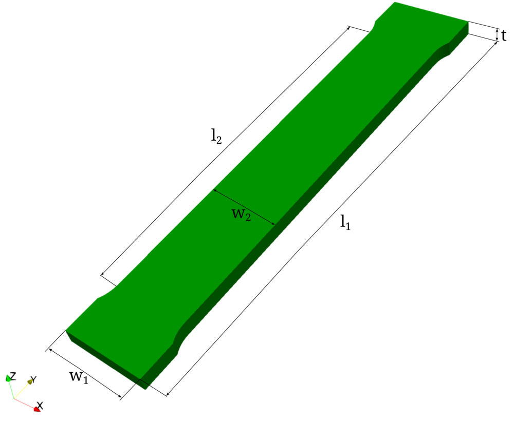
with the measures as listed in the table below
Quantity |
Length in (mm) |
|---|---|
\(l_1\) |
65.0 |
\(l_2\) |
50.0 |
\(w_1\) |
11.34 |
\(w_2\) |
10.0 |
\(t\) |
2.0 |
The material under consideration is an Aluminum alloy with a yield strength of 330 MPa and mild isotropic hardening. During the test, the sample is elongated in the \(y\)-direction and the resulting reaction force is measured.
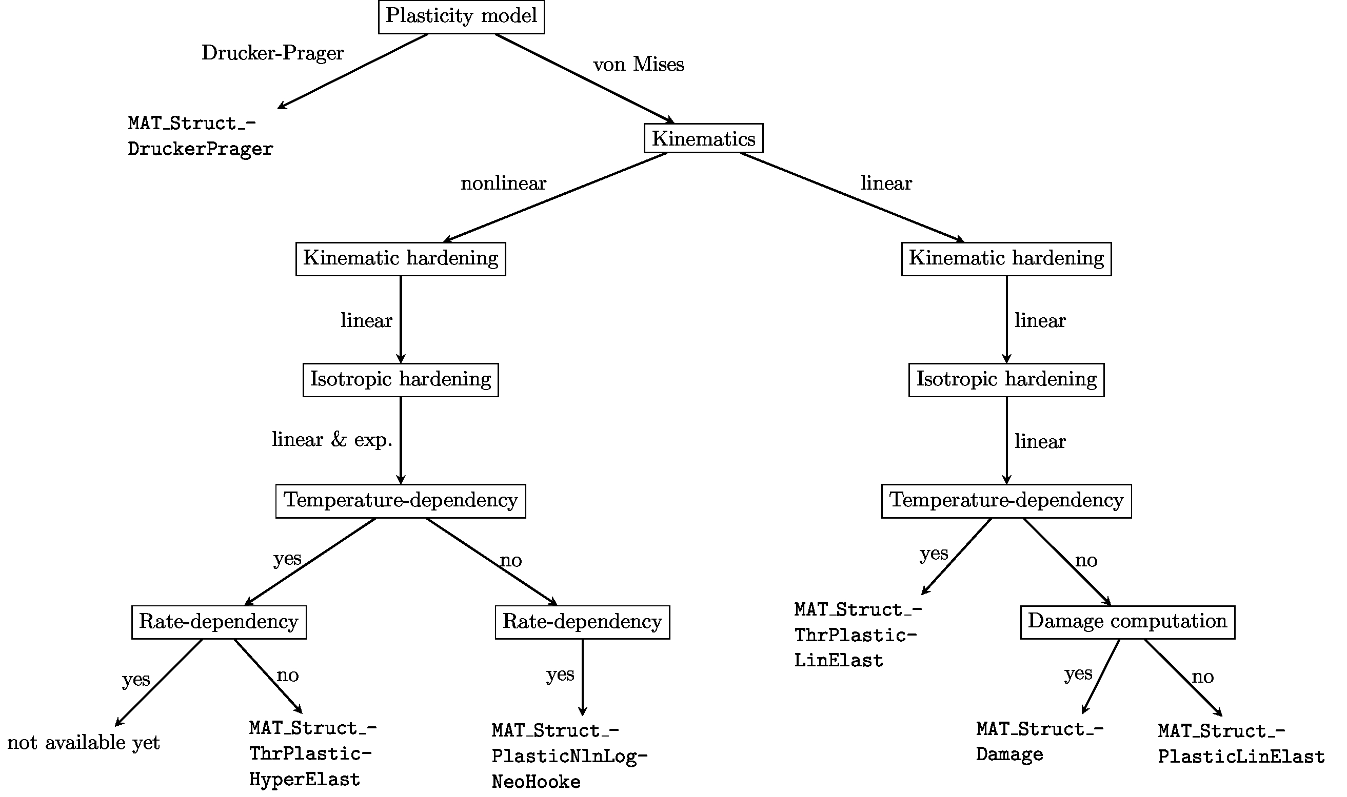
For elasto-plastic simulations 4C provides mainly the following seven material models
MAT_Struct_PlasticLinElast
MAT_Struct_PlasticNlnLogNeoHooke
MAT_Struct_ThermoPlasticHyperElast
MAT_Struct_ThermoPlasticLinElast
MAT_Struct_Damage
MAT_Struct_PlasticGTN
MAT_Struct_DruckerPrager
The following flow chart depicts for which cases these seven models are applicable
|
|---|
Capabilities of plasticity models available in 4C. |
Preprocessing
Due to the symmetry of the problem setup, we may restrict our analysis to one half in the length direction (the \(y\)-direction of the coordinate system).
In addition, symmetry in the width direction (the \(x\)-direction of the coordinate system) and thickness direction (the \(z\)-direction of the coordinate system) can be exploited to reduce the investigated size of the model to one eighth of its original size.
The resulting geometry is discretized with hexahedral elements with quadratic shape functions (HEX27).
In this tutorial, three meshes with different levels of mesh refinement are provided to investigate the spatial convergence of the results.
They are provided in the Exodus II file format following the name pattern: tutorial_solid_geo_<Name>.e, where <Name> needs to be substituted by the names given in the table below.
The table presents properties of the different meshes
Name |
Number of elements |
Number of nodes |
|---|---|---|
coarse |
330 |
3375 |
intermediate |
1400 |
13203 |
fine |
3744 |
33259 |
The mesh of the fine discretization used in this tutorial is shown in the figure below.
|
|---|
Mesh including symmetry assumptions to reduce the model size. Furthermore, the symmetry and displacement boundary conditions are visualized. |
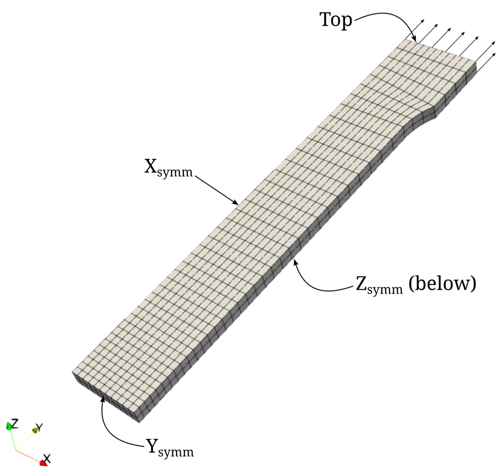
Symmetry boundary conditions are applied to the three symmetry planes, denoted with \(\text{X}_\text{symm}\), \(\text{Y}_\text{symm}\), and \(\text{Z}_\text{symm}\) in the figure above.
The top surface (Top) is subject to a Dirichlet boundary condition with linearly increasing displacement in the positive \(y\)-direction, as displayed in the figure.
The geometry, finite element mesh and node sets for the boundary conditions have been created using Coreform Cubit® .
The corresponding journal file can be run to reproduce this mesh and output a binary EXODUS mesh information file, e.g., tutorial_solid_geo_coarse.e.
The geometry dimensions (actually mainly the radius, all other dimensions depend on it) and element size can be varied, since they are parametrized in the journal file tutorial_solid.jou.
Working with 4C
Creation of a valid 4C input file
To simulate the described problem using 4C, we need to create a valid 4C input file.
A valid template input file for this problem is already provided with the file tutorial_solid.4C.yaml.
In the following, we will briefly walk you through the main settings defined in this input file.
Note
Consider using an IDE like VS Code or Clion to open the 4C input files.
These IDEs can be set up to use the JSON Schema file provided by 4C.
This can be very helpful as it enables to display the documentation of the parameters, allows for auto completion, and shows the different options that can be set.
The file ending of the 4C input files is .4C.yaml.
Note
The documentation of the input parameters can also be very helpful to adapt the input files.
The template input file begins with the following lines
PROBLEM TYPE:
  PROBLEMTYPE: Structure
PROBLEM SIZE:
  DIM: 3
STRUCTURE GEOMETRY:
  FILE: tutorial_solid_geo_coarse.e
  SHOW_INFO: detailed_summary
  ELEMENT_BLOCKS:
  - ID: 1
    SOLID:
      HEX27:
        MAT: 1
        KINEM: nonlinear
in which it is defined that a solid mechanics problem shall be solved (PROBLEMTYPE: Structure) in a three-dimensional setting (DIM: 3).
The last block (STRUCTURE GEOMETRY) defines how the discretized geometry is provided to the code.
It is defined that the mesh shall be read from the file tutorial_solid_geo_coarse.e, which consists of one block of elements, i.e., all elements that define the geometry shown above.
It is further specified that hexahedral elements with quadratic shape functions are used (HEX27), the material with ID 1 is assigned to those elements (MAT: 1), and nonlinear kinematics employing the Green–Lagrange strains are used for the calculations (KINEM: nonlinear).
Moreover, settings for the solid solver need to be set. This is accomplished with the following lines within the input file
STRUCTURAL DYNAMIC:
  INT_STRATEGY: Standard
  DYNAMICTYPE: Statics
  TIMESTEP: 0.2
  RESTARTEVERY: 60
  NUMSTEP: 5
  MAXTIME: 12.0
  TOLDISP: 0.0001
  TOLRES: 0.0001
  PREDICT: TangDis
  LINEAR_SOLVER: 2
Here, the time integration scheme is set to statics, as we investigate a quasi-static problem setup (DYNAMICTYPE: Statics).
Furthermore, the base simulation settings consist of 60 time steps spanning from \(t_0=0\) s to \(t_1=12\) s (MAXTIME) with a time step size of \(\Delta t=0.2\) s (TIMESTEP).
Moreover, the tolerance for the 2-norm of the residual (TOLRES) and the 2-norm of the displacement increments (TOLDISP) is set.
Finally, the linear solver is chosen as the solver with ID 1.
The solver will be defined later in the file by specifying SOLVER 1.
Note
The number of time steps NUMSTEP is set to 5 in the template file to keep the simulation time short for the CI/CD tests.
If you want to run the whole simulation including necking of the specimen, you have to change the parameter to at least NUMSTEP: 60.
The next block of input file lines defines how often and what kind of output is written to visualize the results of the simulations.
IO:
  STRUCT_STRESS: Cauchy
  STRUCT_STRAIN: GL
IO/RUNTIME VTK OUTPUT:
  INTERVAL_STEPS: 1
IO/RUNTIME VTK OUTPUT/STRUCTURE:
  OUTPUT_STRUCTURE: true
  DISPLACEMENT: true
  STRESS_STRAIN: true
IO/MONITOR STRUCTURE DBC:
  INTERVAL_STEPS: 1
First, it is defined that the stress output should be Cauchy stresses (STRUCT_STRESS: Cauchy) and the strain output should be Green–Lagrange strains (STRUCT_STRAIN: GL), while INTERVAL_STEPS: 1 describes the output frequency, i.e., that output in every time step should be performed.
Moreover, the settings in IO/RUNTIME VTK OUTPUT/STRUCTURE activate the output of the solid mechanics solution and define that the displacement field, the stresses, and the strains should be written to output.
The next aspect to be defined is the material definition, which is chosen as follows
MATERIALS:
- MAT: 1
  MAT_Struct_PlasticNlnLogNeoHooke:
    YOUNG: 70000
    NUE: 0.33
    DENS: 1
    YIELD: 330
    SATHARDENING: 1000
    HARDEXPO: 5
    VISC: 0.01
    RATE_DEPENDENCY: 1
Only the material with material ID 1 has been referenced above in the definition of the underlying mesh for the simulation.
Thus, only one material needs to be defined which is called MAT_Struct_PlasticNlnLogNeoHooke.
It is a plasticity model that uses the von Mises yield criterion
with \(\tilde{\mathbf{\tau}}\) being the deviatoric Kirchhoff stress. Additionally, a compressible Neo-Hooke elasticity model is expressed by the free energy. The potential
Here, \(J\) is the determinant of the deformation gradient \(\mathbf{F}\), \(\mathbf{B}^e = \mathbf{F}^e {\mathbf{F}^e}^T\) is the elastic part of the left Cauchy–Green tensor, and \(K, \mu\) are elastic constants. Plasticity with isotropic hardening is assumed
with \(\sigma_{Y,0}=330, \sigma_{Y,\infty} = 1000, k=5\).
Moreover, a Young’s modulus of 70.0e3 and a Poisson’s ratio of 0.33 is prescribed.
Please note, as we are investigating a quasi-static simulation scenario and the time integration Statics is used, dynamic effects and thus the density of the material do not have an effect.
It is thus set to an arbitrary value of 1 in this case.
Furthermore, two linear solvers are defined in the template as follows
SOLVER 1:
  SOLVER: Superlu
  NAME: direct_solver
SOLVER 2:
  SOLVER: Belos
  SOLVER_XML_FILE: iterative_gmres_template.xml
  AZPREC: MueLu
  PRECONDITIONER_XML_FILE: elasticity_template.xml
  NAME: iterative_solver
The SOLVER 1 is the direct solver Superlu.
In addition, an iterative solver, that usually outperforms direct solvers especially for larger systems, is defined as SOLVER 2.
However, a proper setup of an iterative solver is more intricate than just defining a direct solver.
If you want more information on iterative solvers, please refer to the respective tutorial.
At this stage, everything besides the boundary conditions is defined. This is done using the following lines of the input file
DESIGN SURF DIRICH CONDITIONS:
- E: 1
  NUMDOF: 3
  ENTITY_TYPE: node_set_id
  ONOFF:
  - 0
  - 1
  - 0
  VAL:
  - 0
  - 0
  - 0
  FUNCT:
  - 0
  - 0
  - 0
- E: 2
  NUMDOF: 3
  ENTITY_TYPE: node_set_id
  ONOFF:
  - 0
  - 0
  - 1
  VAL:
  - 0
  - 0
  - 0
  FUNCT:
  - 0
  - 0
  - 0
- E: 3
  NUMDOF: 3
  ENTITY_TYPE: node_set_id
  ONOFF:
  - 1
  - 0
  - 0
  VAL:
  - 0
  - 0
  - 0
  FUNCT:
  - 0
  - 0
  - 0
- E: 4
  NUMDOF: 3
  ENTITY_TYPE: node_set_id
  ONOFF:
  - 0
  - 1
  - 0
  VAL:
  - 0
  - 1
  - 0
  FUNCT:
  - 0
  - 1
  - 0
  TAG: monitor_reaction
FUNCT1:
- SYMBOLIC_FUNCTION_OF_SPACE_TIME: t
We briefly describe the definition of the Dirichlet boundary conditions (DBC) applied to the system.
The name DESIGN SURF DIRICH CONDITIONS already describes that the DBC is applied to the surfaces of the geometry.
The component NUMDOF: 3 defines that there are three degrees of freedom (DOF) per node.
Moreover, the component ONOFF is a list of values (one for each DOF) that defines whether the DBC is activated for this DOF (1) or not (0).
The component VAL defines what value is prescribed for the respective DOF.
In addition, a functional expression can be prescribed via FUNCT.
In this case, the prescribed value is calculated based on a multiplication of the evaluated function and the respective constant value in VAL.
Moreover, for the last DBC, the parameter TAG: monitor_reaction is set, which results in tracking the reaction force at that surface.
In the above section, four DBCs are defined.
The following table lists which entity ID (E) belongs to which surface defined in the mesh, as displayed in the picture above
Entity ID ( |
Surface |
|---|---|
1 |
\(\text{Y}_\text{symm}\) |
2 |
\(\text{Z}_\text{symm}\) |
3 |
\(\text{X}_\text{symm}\) |
4 |
Top |
So for the DBC applied to the nodes of the Top surface the following values are prescribed in positive \(y\)-direction
\(1*t\)
originating from the components of (VAL*FUNCT1).
Note
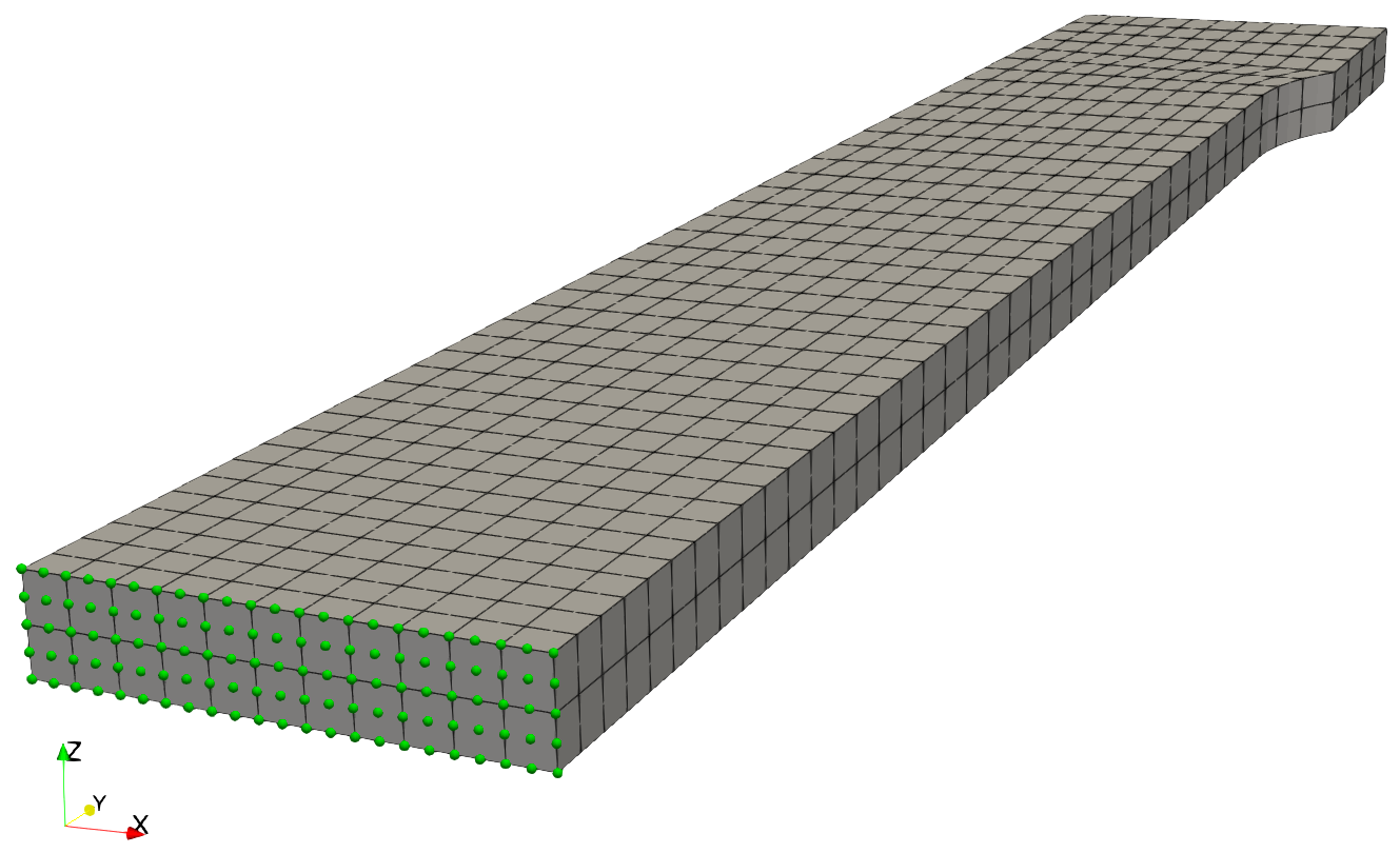
If you want to have a visual impression of what DBC is assigned to which surface of the problem, you can use ParaView.
To do so, open the respective Exodus file in ParaView by: File->Open->Navigate to the desired *.e file and open it.
When activating the checkmark for the node set to be visualized in the Properties tab, the nodes of the selected node set are displayed in RenderView.
The available node sets in the provided geometry files are: xsymm, ysymm, zsymm, and top.
|
|---|
Nodes that are part of the node set of the |
Execute a 4C simulation
Now that the input file for 4C has been created and discussed, the simulation can be started. For execution on a single processor, the simulation is started by the following command
<path-to-build-dir>/4C <path-to-input-file-dir>/tutorial_solid.4C.yaml <path-to-output-file-dir>/tutorial_solid
So first, the location of the executable 4C needs to be given.
Then, the location of the input file and the desired location of the output files need to be specified.
Please note that the <path-to-input-file-dir>/ and the <path-to-output-file-dir>/ can be empty.
In this case, the input file must be in your current working directory, and the output files will be generated in the same directory.
For parallel execution of the simulation using several processes, use
mpirun -np <n_cpu> <path-to-build-dir>/4C <path-to-input-file-dir>/tutorial_solid.4C.yaml <path-to-output-file-dir>/tutorial_solid
meaning that the command mpirun -np <n_cpu> has to be prepended to the original command to specify the number of processors (n_cpu) that should be used.
Note
The screen output during the solution process is rather long but might contain relevant information.
So you can store it in a separate file.
To do so, append |tee <path-to-output-file-dir>/tutorial_solid.txt to the aforementioned commands to store the screen output to the defined txt-file.
Post processing
The results are written in VTK format as defined in the input file.
You will find the following file and directory structure in the output directory (<path-to-output-file-dir>) defined for the execution of 4C:
tutorial_solid.pvd: This ParaView Data file contains the information on where the actual VTK data is stored. When used with e.g. ParaView, only this file needs to be opened to load the complete simulation output data for visualization.tutorial_solid-vtk-files: This is the directory containing the actual output files. Two different file types are created:*.pvtu: For each time step, onepvtufile is created that contains the link to thevtufiles of each processor that was included in the calculation*.vtu: Every processor writes the processor-local output data to a specific file, the so-calledvtufile for each time step. This is the file that contains the actual data.
When opening the result data with e.g. ParaView, the following steps are necessary:
File → Open → Navigate to your output folder and choose the
pvd-file.The filter
Warp By Vectorneeds to be applied to display the specimen in the deformed configuration. Filters → Alphabetical → Warp By VectorDifferent quantities like the displacement field can be chosen from a dropdown menu, and further filters, e.g., to extract specific parts of the complete specimen, or plot certain quantities, can be applied.
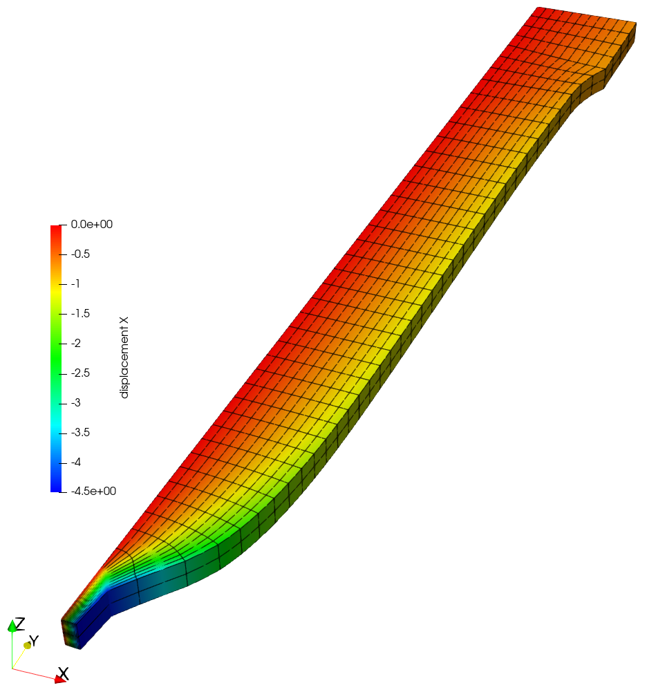
As an example the figure below shows the displacement in \(x\)-direction at the last simulated time step for the mesh with the finest mesh resolution.
|
|---|
Deformed mesh at the last time step with contours of the displacement in \(x\)-direction. |
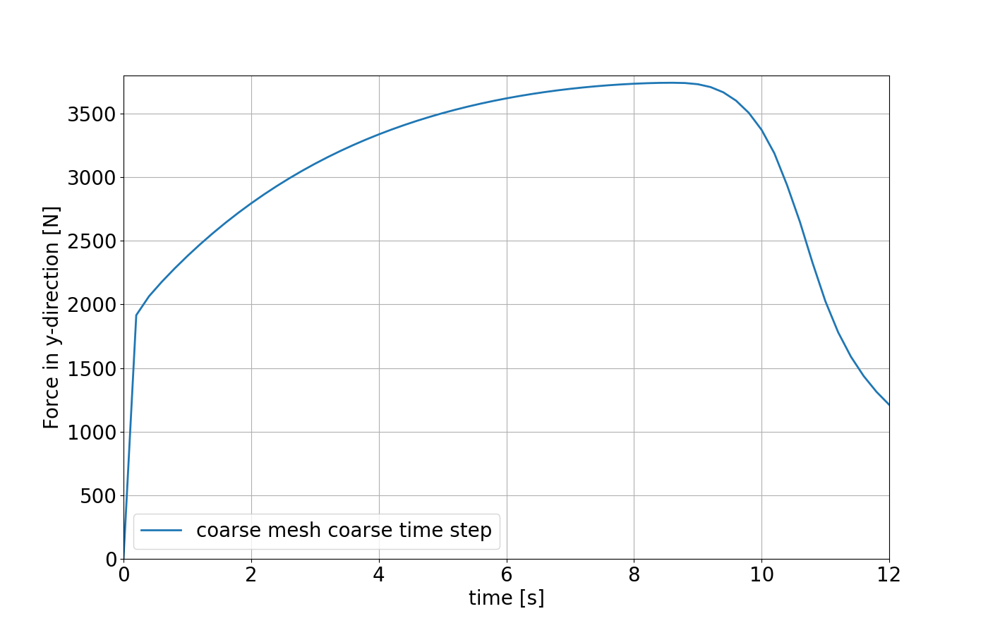
Furthermore, a csv file containing the reaction force of the DBC assigned to the Top surface is written.
For visualizing the reaction force over time ,e.g., a simple python script can be used to obtain
|
|---|
Reaction force of the DBC assigned to the |
Such a python script can be composed of the following commands:
import pandas as pd
import matplotlib.pyplot as plt

# define columns to load from the csv file
columns = ["time", "f:1"]

# load the data
coarse = pd.read_csv(
    "/path/to/csv/file/tutorial_solid-10005_monitor_dbc.csv",
    usecols=columns,
)
# replace one column name as 'f:1' is not accepted for plotting
coarse = coarse.rename(columns={"f:1": "f_y"})

# add the data to the plot
plt.plot(coarse.time, coarse.f_y)

# create the plot
plt.xlabel("time [s]")
plt.ylabel("Force in y-direction [N]")
plt.show()
Numerical analyses
Step 1
We first want to analyze the influence of the chosen solver. In the template 4C input file two solvers have been prepared
SOLVER 1: direct solverSOLVER 2: iterative solver
First, the influence of the solvers on the runtime of the simulations is compared to decide which solver should be used for the subsequent simulations. Please note, that this is also dependent on what mesh is used.
Note
Make sure to choose reasonable names as the simulation output name. Also consider to structure your output data using different directories.
Note
Different meshes result in a different number of degrees of freedom. Thus, it is also recommended to use a different number of processors. The reference results have been produced with
Name |
Number of processors |
|---|---|
coarse |
2 |
intermediate |
4 |
fine |
8 |
Also avoid using the direct solver for the fine mesh as the runtime will be too long.
Solution
To change the used solver from the iterative solver to the direct solver only the definition of the LINEAR_SOLVER in the STRUCTURAL DYNAMIC section needs to be changed from 2 to 1, see below
STRUCTURAL DYNAMIC:
  LINEAR_SOLVER: 1
To change the mesh used in the simulation, only the filename of the parameter FILE in the section STRUCTURE GEOMETRY needs to be changed.
The available meshes are: tutorial_solid_geo_coarse.e, tutorial_solid_geo_intermediate.e, and tutorial_solid_geo_fine.e.
STRUCTURE GEOMETRY:
  FILE: tutorial_solid_geo_intermediate.e
When analyzing the runtimes of the simulations for the direct solver and the iterative solver for the different meshes you can, e.g., compare the screen output Total wall time for CALCULATION: xxx sec of each simulation.
Result
The simulations with the iterative solver are faster for the intermediate and fine meshes and comparable for the coarse mesh.
Thus, the following simulations should be performed with the iterative solver (SOLVER 2).
Step 2
Now, it should be evaluated whether the numerical results are temporally and spatially converged w.r.t. the progression of the reaction force at the DBC over time.
Step 2.1
For the analysis if spatial convergence w.r.t. the progression of the reaction force at the DBC over time is already achieved, three different meshes have been prepared as outlined above.
Since for Step 1 simulations with all meshes have already been performed, the results of these simulation can just be evaluated, e.g., based on the Python commands presented in the section post processing.
Solution
|
|---|
Reaction force of the DBC assigned to the |
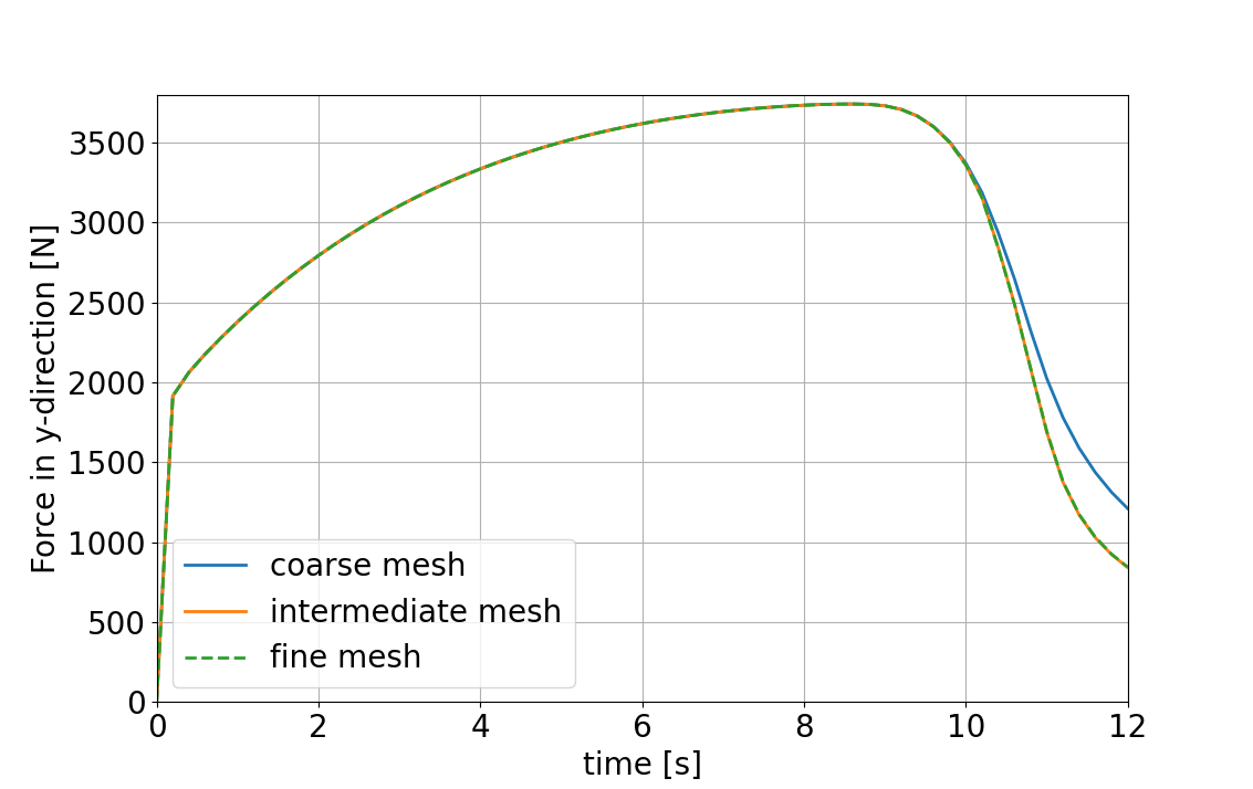
The plot shows no significant changes in the progression of the reaction force over time for the intermediate and fine mesh.
Thus, we consider the simulation to be spatially converged w.r.t. this output quantity for the intermediate mesh.
Step 2.2
To analyze whether temporal convergence concerning the progression of the reaction force at the DBC over time has already been achieved, three different time step sizes are suggested to keep the investigation in a manageable time frame. Thus, the suggested time step sizes for the analysis are: \(0.2\) s (value from the template), \(0.15\) s, and \(0.075\) s.
Solution
To adapt the time step size for the simulations, the parameter TIMESTEP from the section STRUCTURAL DYNAMIC has to be changed.
Note
The parameter NUMSTEP needs to be changed accordingly, such that the desired simulation time MAXTIME is still reached.
Thus, NUMSTEP must be choses such that NUMSTEP * TIMESTEP = MAXTIME holds.
STRUCTURAL DYNAMIC:
  TIMESTEP: 0.15
  NUMSTEP: 80
|
|---|
Reaction force of the DBC assigned to the |
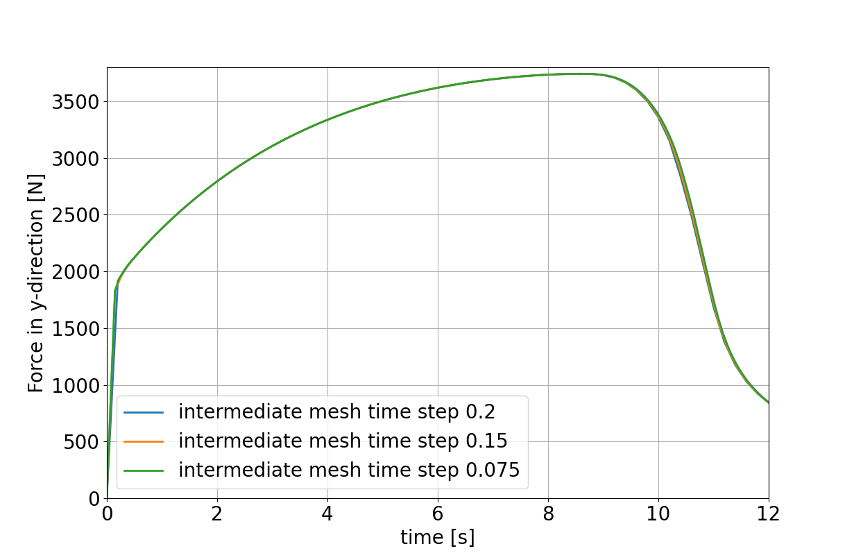
The plot shows no significant changes in the progression of the reaction force over time for the three different time step sizes. Thus, we consider the simulation to be temporally converged w.r.t. this output quantity for all time step sizes.