FSI Tutorial using monolithic approach

This tutorial demonstrates the simulation of a fluid/solid interaction (FSI) problem using a monolithic approach. FSI describes the two-way coupled interaction of solid bodies with fluid flow. A detailed introduction to all flavors of FSI is way beyond the scope of this tutorial. To this end, this tutorial focuses on the following scenario: the solid domain is governed by the equations of elastodynamics, while the flow domain is subject to incompressible Navier-Stokes equations described by an Arbitrary Lagrangean-Eulerian (ALE) observer.

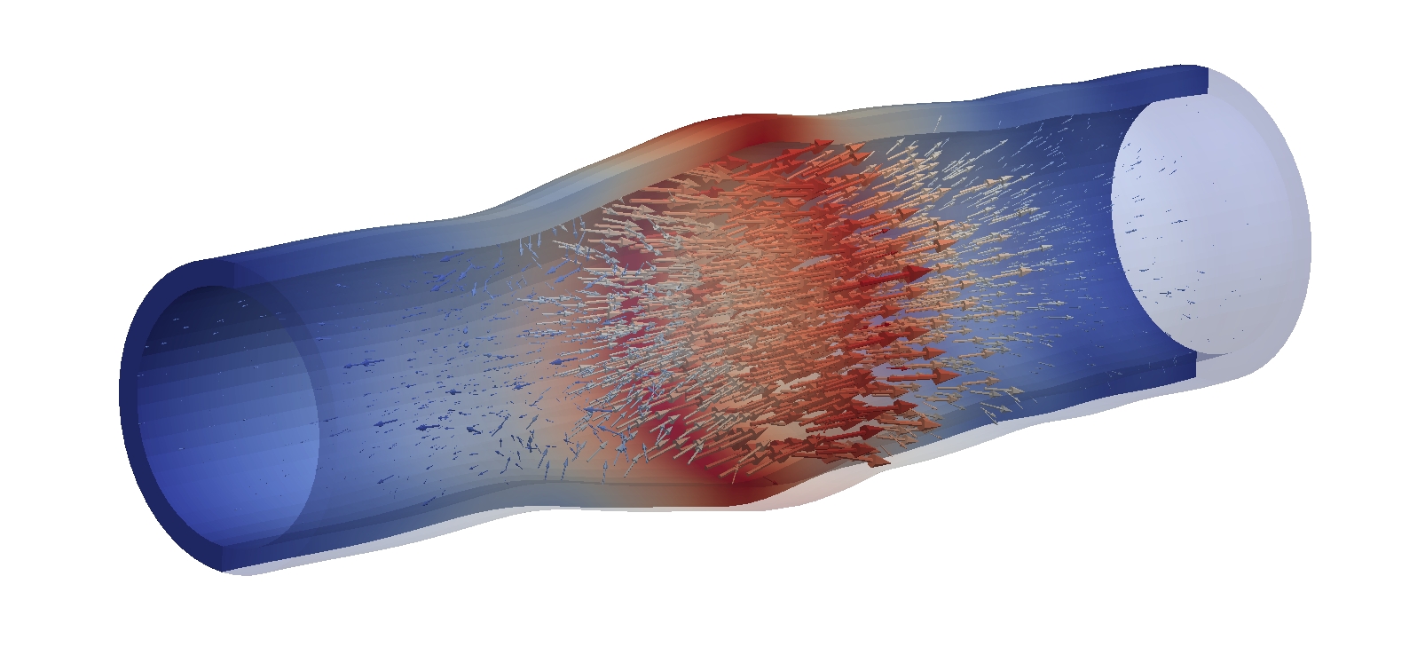
As a concrete example, this tutorial studies a pressure wave through an elastic tube. The tube is clamped at both ends and fully filled with fluid. Both solid and fluid are initially at rest. As external excitation, a pressure pulse is applied to one of the fluid’s boundary cross sections, resulting in a pressure wave traveling along the longitudinal axis of the tube. This also causes a traveling radial expansion of the tube traveling in line with the pressure wave. This problem has originally been introduced in [1] and is designed to mimic hemodynamic conditions, especially w.r.t. to the material densities with the ratio \(\rho^S/\rho^F \approx 1\). Nowadays, it is widely considered a benchmark for monolithic solvers in the FSI community.

Learning objectives

After completion of this tutorial, you will know

• how to set up an FSI problem in 4C;

• how to define meshes, materials, and boundary conditions;

• how to solve the arising linear system with direct and iterative solvers;

• how to interpret the results (pressure wave propagation in an elastic tube).

Therefore, the tutorial will guide you through the process of creating a 4C input file from scratch. For comparison, a working input file fsi/tutorial_fsi_monolithic.4C.yaml is provided in <4C-sourcedir>/tests/tutorials/.

Problem description

The system consists of a straight, thin-walled solid tube (length \(\ell = 5 \mathrm{cm}\), outer radius \(r_o = 0.6 \mathrm{cm}\), inner radius \(r_i = 0.5 \mathrm{cm}\)) that is filled with fluid. The solid tube is fully clamped at both ends. Both solid and fluid are initially at rest.

As external excitation, the fluid surface at \(z = 0\) is loaded with a surface traction \(h^F = 1.3332\cdot 10^4 \mathrm{g \cdot cm/s^2}\) in \(z\)-direction for the duration of \(3\cdot 10^{−3} \mathrm{s}\).

The pressure pulse travels along the longitudinal axis of the tube, causing a traveling radial dilation of the tube:

A detailed analysis of mesh dependence and time integration schemes as well as a series of snapshots of the solution as well as plots for displacement and pressure over time obtained with 4C can be found in [2],[3].

Model setup in 4C

To create a 4C model and input file, at least two ingredients are required:

• The finite element mesh in a suitable mesh format

• A *.4C.yaml file with all simulation parameters and boundary conditions

This tutorial comes with ready-to-use mesh files, so that the focus can be put on creating input files for 4C simulations. In the next steps, you will create your own 4C input file with all necessary simulation parameters, material definitions and boundary conditions and link it to existing finite element mesh files.

Predefined mesh files

This tutorial comes with a series of ready-to-use meshes with different mesh resolutions which can be found in <4C-sourcedir>/tests/tutorials/fsi/. The following meshes are available (along with a recommendation for the number of MPI ranks to run each mesh):

Filename	Global number of DOFs	MPI ranks
tutorial_fsi_monolithic_pw_m1.exo	58333	2
tutorial_fsi_monolithic_pw_m2.exo	187516	8

Each mesh file contains both solid and fluid mesh. The mesh for the mesh motion problem will be generated at run time (see On-the-fly generation of ALE mesh). See for example the mesh tutorial_fsi_monolithic_pw_m1.exo:

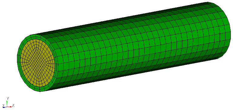
The solid domain is colored in green, the fluid domain in yellow. Note the non-matching grids at the fluid/solid interface.

The mesh contains the following node sets:

Node Set ID	Node Set Name	Description
1	solid_fsi_surf	FSI interface of the solid domain
2	fluid_fsi_surf	FSI interface of the fluid domain
3	solid_clamp_surf	Fully constrained solid surfaces at both ends of the tube
4	fluid_inflow_surf	Fluid surface subject to the pressure pulse
5	fluid_outflow_surf	Fluid surface at the other end of the tube
6	solid_fsi_no_dbc_curves	Solid nodes at the intersection of Dirichlet boundary and FSI interface (not relevant for this tutorial)
7	fluid_fsi_no_dbc_curves	Fluid nodes at the intersection of Dirichlet boundary and FSI interface (not relevant for this tutorial)

Both solid and fluid are meshed with eight-noded hexahedral elements to support a finite element basis with 1st order Lagrange polynomials.

Creating the 4C input file

You can now create the 4C input file. Therefore, create a new file entitled pw.4C.yaml. Now, insert the first set of simulation parameters:

• Define the problem type in order to solve a fluid/solid interaction problem:

PROBLEM TYPE:
  PROBLEMTYPE: Fluid_Structure_Interaction

• Define the spatial dimension:

PROBLEM SIZE:
  DIM: 3

Defining single fields

In order to solve an FSI problem, you now need to define the involved single fields (solid, fluid, ALE mesh motion) as well as the interaction among them. First, let’s define the individual fields:

Define the solid field and time integration strategy

Core parameters for the solid field and time integration strategy are given in the list STRUCTURAL DYNAMIC:

STRUCTURAL DYNAMIC:
  INT_STRATEGY: Old
  LINEAR_SOLVER: 1

The INT_STRATEGY: "Old" points the solid field towards the implementation of solid time integration schemes, that is ready for FSI problems. For a field to be fully defined, it needs to define a LINEAR_SOLVER by referring to a solver section, in this case 1, that will be defined later. In this tutorial, we rely on the solid’s default time integration scheme, Generalized-Alpha time integration with a spectral radius of 1.0 [4].

Note

Link to documentation: See the solid time integration documentation for details and further options.

Define a fluid field and time integration strategy

Core parameters for the fluid field and time integration strategy are given in the list FLUID DYNAMIC:

FLUID DYNAMIC:
  LINEAR_SOLVER: 1
  NONLINITER: Newton
  TIMEINTEGR: Np_Gen_Alpha
  ALPHA_M: 0.5
  ALPHA_F: 0.5
  GAMMA: 0.5
  GRIDVEL: BDF2

Similar to the solid field, a default LINEAR_SOLVER must be defined. NONLINITER: Newton instructs the fluid field to assemble all linearization terms, such that the monolithic FSI scheme can solve the nonlinear problem in each time step with a Newton method using a consistent linearization of all residual terms. A 2nd-order backward differentiation formula (BDF2) is used to approximate the grid velocity in the ALE description of the Navier-Stokes equations based on the ALE Mesh displacements. The fluid field performs time integration via the Generalized-alpha scheme [5] with parameters ALPHA_M, ALPHA_F and GAMMA as given.

Note

Link to documentation: See the fluid time integration documentation for details and further options.

Define the ALE mesh motion field

The mesh motion problem of the ALE formulation of the fluid domain is defined as follows:

ALE DYNAMIC:
  ALE_TYPE: springs_material
  LINEAR_SOLVER: 1

The ALE_TYPE specifies the mesh motion algorithm to interpret the mesh as a network of springs. Similar to solid and fluid field, a default LINEAR_SOLVER must be defined.

Defining the FSI coupling interaction

We can now define the FSI algorithm. In particular, we have to specify the FSI coupling algorithms, some aspects of time discretization, as well as details on the coupling iterations.

First, we describe the overall FSI procedure by adding the following lines to the 4C input file:

FSI DYNAMIC:
  COUPALGO: iter_mortar_monolithicfluidsplit
  SECONDORDER: true
  MAXTIME: 0.0005
  TIMESTEP: 0.0001

To enable non-matching grids at the FSI interface with Lagrange multiplier unknowns for constraint enforcement being discretized on the fluid side of the interface, we specify the coupling algorithm COUPALGO as "iter_mortar_monolithicfluidsplit". The setting SECONDORDER: true yields a 2nd order conversion between displacements and velocities at the FSI interface. We then run the simulation with a TIMESTEP of 0.0001 up to a maximum simulation time MAXTIME of 0.001.

Note

We start with a short simulation to get things up and running. Feel free to switch to an extended MAXTIME at a later stage in order to give the pressure wave time to travel through the elastic tube.

For details on the FSI algorithm, see [6],[2].

To solve the nonlinear FSI problem with a monolithic approach, insert the following section:

FSI DYNAMIC/MONOLITHIC SOLVER:
  SHAPEDERIVATIVES: true
  LINEARBLOCKSOLVER: LinalgSolver
  LINEAR_SOLVER: 2
  TOL_DIS_RES_L2: 1e-06
  TOL_DIS_RES_INF: 1e-06
  TOL_DIS_INC_L2: 1e-06
  TOL_DIS_INC_INF: 1e-06
  TOL_FSI_RES_L2: 1e-06
  TOL_FSI_RES_INF: 1e-06
  TOL_FSI_INC_L2: 1e-06
  TOL_FSI_INC_INF: 1e-06
  TOL_PRE_RES_L2: 1e-06
  TOL_PRE_RES_INF: 1e-06
  TOL_PRE_INC_L2: 1e-06
  TOL_PRE_INC_INF: 1e-06
  TOL_VEL_RES_L2: 1e-06
  TOL_VEL_RES_INF: 1e-06
  TOL_VEL_INC_L2: 1e-06
  TOL_VEL_INC_INF: 1e-06

Therein, SHAPEDERIVATIVES: true includes the linearization of fluid residuals with respect to the mesh deformation into the FSI Jacobian matrix [2]. The choice of LINEARBLOCKSOLVER: "LinalgSolver" instructs the monolithic solution scheme to solve the linear system through 4C’s centralized linear solver interface, LinalgSolver, and refers to a linear solver with ID 2 (to be defined later) for the concrete parametrization of the linear solver. The remaining parameters specify the tolerances for the convergence test of the nonlinear solver, that tests convergence of solid displacements, fluid velocities and pressures, as well as interface quantities separately and each in 2- and inf-norm (see Appendix A.1 of [7] for details).

Defining the constitutive behavior of each field

So far, we have defined time integration parameters for the involved solid, fluid, and mesh motion field. Yet, the constitutive behavior of solid and fluid are still missing.

They are defined as follows:

MATERIALS:
- MAT: 1
  MAT_fluid:
    DYNVISCOSITY: 0.03
    DENSITY: 1
- MAT: 2
  MAT_Struct_StVenantKirchhoff:
    YOUNG: 3e+6
    NUE: 0.3
    DENS: 1.2

Thereby, MAT: 1 specifies a Newtonian fluid for the fluid domain, while MAT 2 defines a St.-Venant-Kirchhoff material for the solid domain. The values correspond to the pressure wave example [1].

Note

Link to documentation: For details, see the 4C documentation: Newtonian fluid, St.-Venant-Kirchhoff

Geometry and mesh information

Geometry and mesh information are provided in ready-to-use mesh files for this tutorial.

Note

Link to documentation: A brief introduction to meshes in 4C is given in the preprocessing documentation.

Solid domain and mesh

The solid geometry and its mesh are pre-defined in mesh files, cf predefined mesh files. To use it in a 4C simulation, the input file needs to refer to the solid mesh as follows:

STRUCTURE GEOMETRY:
  FILE: tutorial_fsi_monolithic_pw_m1.exo
  ELEMENT_BLOCKS:
  - ID: 1
    SOLID:
      HEX8:
        MAT: 2
        KINEM: nonlinear
        TECH: eas_full

Therein, FILE: "tutorial_fsi_monolithic_pw_m1.exo" points to the pre-defined mesh file. The solid domain is defined as one of the meshes ELEMENT_BLOCKS, in this case the block with ID: 1. The elements in this block will be finite elements with ELEMENT_NAME: SOLID and ELEMENT_DATA: "MAT 2 KINEM nonlinear TECH eas_full".

Fluid domain and mesh

Similarly, the fluid geometry and mesh is included via:

FLUID GEOMETRY:
  FILE: tutorial_fsi_monolithic_pw_m1.exo
  ELEMENT_BLOCKS:
  - ID: 2
    FLUID:
      HEX8:
        MAT: 1
        NA: ALE

On-the-fly generation of ALE mesh

Meshes for solid and fluid are part of the pre-defined mesh file. It is common practice to use the fluid mesh also for the mesh motion problem. Thus, it can be created from the fluid mesh at run time.

Therefore, insert the following section into the 4C input file:

CLONING MATERIAL MAP:
- SRC_FIELD: fluid
  SRC_MAT: 1
  TAR_FIELD: ale
  TAR_MAT: 2

It specifies to clone a field. Source and target fields are identified via the IDs of their material. In this case, SRC_FIELD: "fluid" with SRC_MAT: 1 is used as the source field. The cloning operation will generate a target field defined by TAR_FIELD: "ale" and will assign it the target material TAR_MAT: 2.

Please keep in mind that the actual stiffness value of the ALE field is irrelevant and does not influence the physical solution. Therefore, it is ok to refer to the solid material here for simplicity.

Boundary conditions

To apply the required boundary and coupling conditions, we will look at each type of boundary condition separately.

To impose a boundary condition, we need to specify not only its type and values, but also the mesh entities of the degrees of freedom that are subject to this boundary condition. A list of relevant mesh entities is given in the table with all node sets of the predefined mesh files.

Essential / Dirichlet boundary conditions

In the pressure wave example, there are only two types of Dirichlet conditions:

• Clamping of the solid tube at both ends

• Fixation of fluid mesh motion at both ends of the tube

We start with the two end surfaces of the solid tube. They are fully clamped, i.e., all three displacements are constrained to zero at the respective surfaces. This can be achieved by defining a DESIGN SURF DIRICH CONDITIONS in the 4C input file:

DESIGN SURF DIRICH CONDITIONS:
- E: 3
  ENTITY_TYPE: node_set_id
  NUMDOF: 3
  ONOFF:
  - 1
  - 1
  - 1
  VAL:
  - 0.0
  - 0.0
  - 0.0
  FUNCT:
  - null
  - null
  - null

Explanation:

• E: 3: This defines the location of the Dirichlet condition, which refers to the list of node sets: all nodes of the solid end surfaces are stored in node set 3.

• ENTITY_TYPE: node_set_id: Adds context that the E: 3 needs to be interpreted as an ID of a node set.

• NUMDOF: 3: The solid field has three degrees of freedom per node.

• ONOFF: [1,1,1]: Activate the Dirichlet boundary condition for each of the degrees of freedom at a node.

• VAL: [0.0,0.0,0.0]: Specify the value of the prescribed displacement for each of the degrees of freedom at a node.

The ALE mesh motion at the fluid cross section areas at both ends of the tube is constrained via DESIGN SURF ALE DIRICH CONDITIONS. Its internal setup is the same as a regular Dirichlet condition (for example such as the one in the solid field), however the addendum of ALE is required since the ALE mesh motion field is not defined in the mesh file, but has been created by cloning the fluid discretization. The boundary condition reads:

DESIGN SURF ALE DIRICH CONDITIONS:
- E: 4
  ENTITY_TYPE: node_set_id
  NUMDOF: 3
  ONOFF:
  - 1
  - 1
  - 1
  VAL:
  - 0.0
  - 0.0
  - 0.0
  FUNCT:
  - null
  - null
  - null
- E: 5
  ENTITY_TYPE: node_set_id
  NUMDOF: 3
  ONOFF:
  - 1
  - 1
  - 1
  VAL:
  - 0.0
  - 0.0
  - 0.0
  FUNCT:
  - null
  - null
  - null

In order to later impose the pressure pulse on only one of the surfaces the fluid cross section areas at both ends of the tube are stored in two different nodes sets. Therefore, the ALE Dirichlet boundary condition must be applied for each of the surfaces, in this case in accordance with the mesh details from the predefined mesh files for E: 4 and E: 5. All other parameters follow the same logic as the Dirichlet boundary condition for the solid field and impose a zero-displacement-condition for all ALE degrees of freedom on the two surfaces.

Flux / Neumann boundary conditions

The pressure pulse onto the fluid will be modeled as a Neumann boundary condition. It acts onto one of the cross section surfaces of the fluid domain. Its definition in the 4C input file reads:

DESIGN SURF NEUMANN CONDITIONS:
- E: 4
  ENTITY_TYPE: node_set_id
  NUMDOF: 4
  ONOFF:
  - 0
  - 0
  - 1
  - 0
  VAL:
  - 0
  - 0
  - -13332
  - 0
  FUNCT:
  - null
  - null
  - 1
  - null

• E: 4: This refers to the node set 4 representing all nodes in one of the two fluid cross sections, see predefined mesh files.

• ENTITY_TYPE: node_set_id: Adds context that the E: 3 needs to be interpreted as an ID of a node set.

• NUMDOF: 4: The three-dimensional flow problem has four degrees of freedom per node, namely three velocities and one pressure unknown.

• ONOFF: [0,0,1,0]: Given the orientation of the tube in the global frame of reference, the external traction must act in negative z-direction of the velocity degrees of freedom. Due to the internal ordering (x-, y-, z-velocities, pressure) of unknows at each fluid node, the third component is activated by setting 1, while all other components remain inactive by setting 0.

• VAL: [0,0,-13332,0]: Following the same argument, only the third component needs to carry an actual value, in this case the value of the traction in negative z-direction.

• FUNCT: [null,null,1,null] specifies the (time-dependent) function FUNCT 1 for the z-component of the external load.

The pressure pulse will be imposed as a peak at the beginning of the simulation. It is modeled as a linear interpolation between user-given values in function FUNCT 1 as follows:

FUNCT1:
- COMPONENT: 0
  SYMBOLIC_FUNCTION_OF_SPACE_TIME: initial_pressure_pulse
- VARIABLE: 0
  NAME: initial_pressure_pulse
  TYPE: linearinterpolation
  NUMPOINTS: 4
  TIMES:
  - 0
  - 0.003
  - 0.0031
  - 10000
  VALUES:
  - 1.0
  - 1.0
  - 0.0
  - 0.0

The linear interpolation is defined by specifying NUMPOINTS: 4 data points at time instances TIMES: [0,0.003,0.0031,10000] with assigned values VALUES: [1.0,1.0,0.0,0.0].

FSI coupling condition

The mesh comes with non-matching grids at the fluid/solid interface. Therefore, we employ a mortar approach to impose the coupling conditions [6],[2].

According to the predefined mesh files, the solid side of the interface is stored in node set 1, while the fluid side of the interface is stored in node set 2. Both sides need to be defined as FSI coupling partners:

DESIGN FSI COUPLING SURF CONDITIONS:
- E: 1
  ENTITY_TYPE: node_set_id
  coupling_id: 1
- E: 2
  ENTITY_TYPE: node_set_id
  coupling_id: 1

Again, E: 1 and E: 2 are the IDs with ENTITY_TYPE: node_set_id instructing to interpret them as node set IDs. The coupling_id: 1 assigns both coupling surfaces to the FSI interface 1.

Linear solver

In this tutorial, we will explore two different solver options for monolithic FSI problesm: direct vs. iterative. While direct solvers are easy to use, since they do not require the choice of solver parameters, they are often less efficient than properly preconditioned iterative linear solvers.

Direct solver

First, we start with a direct solver. It is defined as follows:

SOLVER 1:
  SOLVER: UMFPACK

This enables UMFPACK [8] as direct solver, which will compute an LU factorization of the FSI system matrix and use it to solve the arising linear system of equations.

To tell the FSI algorithm to use this solver, make sure to assign the value 1 to the input parameter LINEAR_SOLVER in the FSI DYNAMIC/MONOLITHIC SOLVER: section of the 4C input file.

Iterative solver with preconditioner

To overcome performance and feasibility limitations of direct solvers, let us now explore iterative solvers with appropriate preconditioning. Therefore, define a second solver in the 4C input file by adding:

SOLVER 2:
  SOLVER: Belos
  AZPREC: MueLu
  AZREUSE: 10
  SOLVER_XML_FILE: iterative_gmres_template.xml
  MUELU_XML_FILE: fluid_solid_ale.xml

The parameter SOLVER: "Belos" enables a Generalized Minimal Residual (GMRES) solver [9] from Trilinos’ Belos package [10] as an iterative solver, which will approximate the solution of the linear system up to a user-given tolerance. The exact settings of the GMRES method are pre-defined in iterative_gmres_template.xml. This file is provided in <4C-sourcedir>/tests/input_files/xml/linear_solver/. To accelerate convergence of the GMRES solver, AZPREC points 4C to use Trilinos’ MueLu package as a preconditioner. In this tutorial, we employ a fully coupled algebraic multigrid preconditioner tailored to FSI systems as proposed in [11]. It is defined in fluid_solid_ale.xml in <4C-sourcedir>/tests/input_files/xml/multigrid/. The 4C repository provides some solver configurations and exemplary configurations for different types of preconditioners in <4C-sourcedir>/tests/input_files/xml/. By setting AZREUSE: 10, the preconditioner can be reused up to ten times in order to save the cost for preconditioner setup.

To tell the FSI algorithm to use SOLVER 2, make sure to assign the value 2 to the input parameter LINEAR_SOLVER in the FSI DYNAMIC/MONOLITHIC SOLVER: section of the 4C input file.

Note

Note on file locations: Support files (such as the solver configuration iterative_gmres_template.xml or the preconditioner configuration fluid_solid_ale.xml) can be placed anywhere. However, the 4C input file needs to refer to these files by either relative or absolute paths. In this tutorial, we assume that these files are in the same directory as the 4C input file pw.4C.yaml.

Note

Link to documentation: For details on the use and definition of iterative solvers and multigrid preconditioners in 4C, we refer to 4C’s preconditioning tutorial.

Running the FSI Simulation

With a complete *.4C.yaml input file at hand, you are now in the position to run the simulation.

Prerequisites

To run a 4C simulation, you need a compiled 4C executable and 4C input data.

• Executable: We assume the 4C build directory to be located at <path/to/build/directory>. The 4C executable is located in this build directory.

• 4C mesh file: For this tutorial, please use one of the pre-defined mesh files tutorial_fsi_monolithic_pw_m*.exo as described in the section on predefined mesh files.

• 4C input file: For this tutorial, please use the input file pw.4C.yaml that you have created in the previous steps, cf. creating the 4C input file. We assume the 4C input to be located at <path/to/input/file>.

Starting a 4C simulation

4C can run in parallel distributed to multiple cores. We denote the number of cores by <numCores> throughout this tutorial.

To write output, the user has to provide an output prefix that is used for all output files. We assume output to be prefixed by <path/to/output>.

To run 4C on <numCores> cores, execute the following command:

mpirun -np <numCores> <path/to/build/directory>/4C <path/to/input/file> <path/to/output>

Postprocessing

For FSI simulations, 4C writes simulation output in binary format. To view it in ParaView, first run the postprocessing as follows:

<path/to/build/directory>/post_ensight --file=<path/to/output>

This will produce a series of files ready for inspection in ParaView. Please consult the ParaView documentation on all questions related to ParaView. Open the two files ending with *_fluid.case and *_structure.case in ParaView. This will load the results of the fluid and solid domain into ParaView. Now, you can inspect the solution in ParaView, apply filters, walk through the different time steps, etc. You now should be able to obtain a visualization like the one in the section on Problem description.

Note

Visualization of deformations: Both solid and fluid domain have computed displacement fields during the simulation. To visualize the deformation, you can

• create a contour plot for each domain colored according to the displacement field of each domain;

• display the deformation of the geometry by applying a “warp” filter. For better visibility, it is recommended to scale the deformation by a factor, e.g. 10 or 100.

Further numerical experiments

So far, we have just run five time steps of the pressure wave example using a medium-sized mesh and direct solver for the linear system. We can now vary some parameters.

Step 1: Switch to iterative solver

An iterative solver, defined as SOLVER 2 in the input file, has already been specified, but has not yet been used so far.

To switch from the direct solver (SOLVER 1) to an iterative solver with multigrid preconditioning (SOLVER 2), we have to point the monolithic FSI configuration to SOLVER 2. This is achieved by setting LINEAR_SOLVER: 2 in the FSI DYNAMIC/MONOLITHIC SOLVER: section of the input file.

Change and save the input file and re-run the FSI example. Observe the screen output.

Solution

For an iterative solver, we first have to create a preconditioner. Its output is a bit lengthy and looks like this:

*******************************************************
Recomputation due to reaching 0 nonlinear steps.
Recomputation due to reset.
Compute preconditioner
*******************************************************
Clearing old data (if any)

Level 0
Setup blocked Gauss-Seidel Smoother (MueLu::BlockedGaussSeidelSmoother{type = blocked GaussSeidel})
Setup Smoother (MueLu::IfpackSmoother{type = Chebyshev})
Build (MueLu::SubBlockAFactory)
A(0,0) is a single block and has strided maps:
  range  map fixed block size = 3, strided block id = -1
  domain map fixed block size = 3, strided block id = -1
chebyshev: max eigenvalue (calculated by Ifpack) = 5.27
"Ifpack Chebyshev polynomial": {Initialized: true, Computed: true, degree: 3, lambdaMax: 5.26514, alpha: 20, lambdaMin: 0.263257}
Setup Smoother (MueLu::IfpackSmoother{type = ILU})
Build (MueLu::SubBlockAFactory)
A(1,1) is a single block and has strided maps:
  range  map fixed block size = 4, strided block id = -1
  domain map fixed block size = 4, strided block id = -1
Ifpack_AdditiveSchwarz, ov = 0, local solver =
		***** `IFPACK ILU (fill=1, relax=0.000000, athr=0.000000, rthr=1.000000)'
       ***** Condition number estimate = 9.58277e+09
Setup Smoother (MueLu::IfpackSmoother{type = Chebyshev})
Build (MueLu::SubBlockAFactory)
A(2,2) is a single block and has strided maps:
  range  map fixed block size = 3, strided block id = -1
  domain map fixed block size = 3, strided block id = -1
chebyshev: max eigenvalue (calculated by Ifpack) = 2.07
"Ifpack Chebyshev polynomial": {Initialized: true, Computed: true, degree: 3, lambdaMax: 2.07381, alpha: 20, lambdaMin: 0.103691}

Level 1
Build (MueLu::BlockedPFactory)
Prolongator smoothing (MueLu::SaPFactory)
Build (MueLu::TentativePFactory)
Build (MueLu::UncoupledAggregationFactory)
Build (MueLu::CoalesceDropFactory)
Build (MueLu::AmalgamationFactory)
lightweight wrap = 1
algorithm = "classical" classical algorithm = "default": threshold = 0.00, blocksize = 3
Detected 144 agglomerated Dirichlet nodes
Number of dropped entries in amalgamated matrix graph: 0/84168 (0.00%)
BuildAggregatesNonKokkos (Phase - (Dirichlet))
  aggregated : 144 (phase), 144/2376 [6.06%] (total)
  remaining  : 2232
  aggregates : 0 (phase), 0 (total)
BuildAggregatesNonKokkos (Phase 1 (main))
  aggregated : 1977 (phase), 2121/2376 [89.27%] (total)
  remaining  : 255
  aggregates : 73 (phase), 73 (total)
BuildAggregatesNonKokkos (Phase 2a (secondary))
  aggregated : 0 (phase), 2121/2376 [89.27%] (total)
  remaining  : 255
  aggregates : 0 (phase), 73 (total)
BuildAggregatesNonKokkos (Phase 2b (expansion))
  aggregated : 255 (phase), 2376/2376 [100.00%] (total)
  remaining  : 0
  aggregates : 0 (phase), 73 (total)
BuildAggregatesNonKokkos (Phase 3 (cleanup))
  aggregated : 0 (phase), 2376/2376 [100.00%] (total)
  remaining  : 0
  aggregates : 0 (phase), 73 (total)
Nullspace factory (MueLu::NullspaceFactory)
Build (MueLu::CoarseMapFactory)
Using cached max eigenvalue estimate
Prolongator damping factor = 0.25 (1.33 / 5.27)
Build (MueLu::TentativePFactory)
Build (MueLu::UncoupledAggregationFactory)
Build (MueLu::CoalesceDropFactory)
Build (MueLu::AmalgamationFactory)
lightweight wrap = 1
algorithm = "classical" classical algorithm = "default": threshold = 0.00, blocksize = 4
Detected 0 agglomerated Dirichlet nodes
Number of dropped entries in amalgamated matrix graph: 0/183031 (0.00%)
BuildAggregatesNonKokkos (Phase - (Dirichlet))
  aggregated : 0 (phase), 0/7315 [0.00%] (total)
  remaining  : 7315
  aggregates : 0 (phase), 0 (total)
BuildAggregatesNonKokkos (Phase 1 (main))
  aggregated : 5643 (phase), 5643/7315 [77.14%] (total)
  remaining  : 1672
  aggregates : 209 (phase), 209 (total)
BuildAggregatesNonKokkos (Phase 2a (secondary))
  aggregated : 0 (phase), 5643/7315 [77.14%] (total)
  remaining  : 1672
  aggregates : 0 (phase), 209 (total)
BuildAggregatesNonKokkos (Phase 2b (expansion))
  aggregated : 1672 (phase), 7315/7315 [100.00%] (total)
  remaining  : 0
  aggregates : 0 (phase), 209 (total)
BuildAggregatesNonKokkos (Phase 3 (cleanup))
  aggregated : 0 (phase), 7315/7315 [100.00%] (total)
  remaining  : 0
  aggregates : 0 (phase), 209 (total)
Nullspace factory (MueLu::NullspaceFactory)
Build (MueLu::BlockedCoarseMapFactory)
Prolongator smoothing (MueLu::SaPFactory)
Build (MueLu::TentativePFactory)
Build (MueLu::UncoupledAggregationFactory)
Build (MueLu::CoalesceDropFactory)
Build (MueLu::AmalgamationFactory)
lightweight wrap = 1
algorithm = "classical" classical algorithm = "default": threshold = 0.00, blocksize = 3
Detected 354 agglomerated Dirichlet nodes
Number of dropped entries in amalgamated matrix graph: 0/147765 (0.00%)
BuildAggregatesNonKokkos (Phase - (Dirichlet))
  aggregated : 354 (phase), 354/6195 [5.71%] (total)
  remaining  : 5841
  aggregates : 0 (phase), 0 (total)
BuildAggregatesNonKokkos (Phase 1 (main))
  aggregated : 3834 (phase), 4188/6195 [67.60%] (total)
  remaining  : 2007
  aggregates : 142 (phase), 142 (total)
BuildAggregatesNonKokkos (Phase 2a (secondary))
  aggregated : 0 (phase), 4188/6195 [67.60%] (total)
  remaining  : 2007
  aggregates : 0 (phase), 142 (total)
BuildAggregatesNonKokkos (Phase 2b (expansion))
  aggregated : 2007 (phase), 6195/6195 [100.00%] (total)
  remaining  : 0
  aggregates : 0 (phase), 142 (total)
BuildAggregatesNonKokkos (Phase 3 (cleanup))
  aggregated : 0 (phase), 6195/6195 [100.00%] (total)
  remaining  : 0
  aggregates : 0 (phase), 142 (total)
Nullspace factory (MueLu::NullspaceFactory)
Build (MueLu::BlockedCoarseMapFactory)
Using cached max eigenvalue estimate
Prolongator damping factor = 0.64 (1.33 / 2.07)
Call prolongator factory for calculating restrictor (MueLu::GenericRFactory)
Build (MueLu::BlockedPFactory)
Transpose P (MueLu::TransPFactory)
Transpose P (MueLu::TransPFactory)
Transpose P (MueLu::TransPFactory)
Computing Ac (block) (MueLu::BlockedRAPFactory)
Setup blocked Gauss-Seidel Smoother (MueLu::BlockedGaussSeidelSmoother{type = blocked GaussSeidel})
Setup Smoother (MueLu::IfpackSmoother{type = Chebyshev})
Build (MueLu::SubBlockAFactory)
A(0,0) is a single block and has strided maps:
  range  map fixed block size = 6, strided block id = -1
  domain map fixed block size = 6, strided block id = -1
chebyshev: ratio eigenvalue (computed) = 125.51
chebyshev: max eigenvalue (calculated by Ifpack) = 1.31
"Ifpack Chebyshev polynomial": {Initialized: true, Computed: true, degree: 3, lambdaMax: 1.31462, alpha: 125.509, lambdaMin: 0.0104743}
Setup Smoother (MueLu::IfpackSmoother{type = ILU})
Build (MueLu::SubBlockAFactory)
A(1,1) is a single block and has strided maps:
  range  map fixed block size = 4, strided block id = -1
  domain map fixed block size = 4, strided block id = -1
Ifpack_AdditiveSchwarz, ov = 0, local solver =
       ***** `IFPACK ILU (fill=1, relax=0.000000, athr=0.000000, rthr=1.000000)'
       ***** Condition number estimate = 3.05621e+10
Setup Smoother (MueLu::IfpackSmoother{type = Chebyshev})
Build (MueLu::SubBlockAFactory)
A(2,2) is a single block and has strided maps:
  range  map fixed block size = 6, strided block id = -1
  domain map fixed block size = 6, strided block id = -1
chebyshev: ratio eigenvalue (computed) = 64.52
chebyshev: max eigenvalue (calculated by Ifpack) = 1.52
"Ifpack Chebyshev polynomial": {Initialized: true, Computed: true, degree: 3, lambdaMax: 1.52467, alpha: 64.5223, lambdaMin: 0.0236301}

Level 2
Build (MueLu::BlockedPFactory)
Prolongator smoothing (MueLu::SaPFactory)
Build (MueLu::TentativePFactory)
Build (MueLu::UncoupledAggregationFactory)
Build (MueLu::CoalesceDropFactory)
PreDropFunctionConstVal: threshold = 0
Build (MueLu::AmalgamationFactory)
lightweight wrap = 1
algorithm = "classical" classical algorithm = "default": threshold = 0.00, blocksize = 6
Detected 0 agglomerated Dirichlet nodes
Number of dropped entries in amalgamated matrix graph: 0/3347 (0.00%)
BuildAggregatesNonKokkos (Phase - (Dirichlet))
  aggregated : 0 (phase), 0/73 [0.00%] (total)
  remaining  : 73
  aggregates : 0 (phase), 0 (total)
BuildAggregatesNonKokkos (Phase 1 (main))
  aggregated : 72 (phase), 72/73 [98.63%] (total)
  remaining  : 1
  aggregates : 2 (phase), 2 (total)
BuildAggregatesNonKokkos (Phase 2a (secondary))
  aggregated : 0 (phase), 72/73 [98.63%] (total)
  remaining  : 1
  aggregates : 0 (phase), 2 (total)
BuildAggregatesNonKokkos (Phase 2b (expansion))
  aggregated : 1 (phase), 73/73 [100.00%] (total)
  remaining  : 0
  aggregates : 0 (phase), 2 (total)
BuildAggregatesNonKokkos (Phase 3 (cleanup))
  aggregated : 0 (phase), 73/73 [100.00%] (total)
  remaining  : 0
  aggregates : 0 (phase), 2 (total)
Nullspace factory (MueLu::NullspaceFactory)
Build (MueLu::CoarseMapFactory)
Using cached max eigenvalue estimate
Prolongator damping factor = 1.01 (1.33 / 1.31)
Build (MueLu::TentativePFactory)
Build (MueLu::UncoupledAggregationFactory)
Build (MueLu::CoalesceDropFactory)
PreDropFunctionConstVal: threshold = 0
Build (MueLu::AmalgamationFactory)
lightweight wrap = 1
algorithm = "classical" classical algorithm = "default": threshold = 0.00, blocksize = 4
Detected 0 agglomerated Dirichlet nodes
Number of dropped entries in amalgamated matrix graph: 0/3275 (0.00%)
BuildAggregatesNonKokkos (Phase - (Dirichlet))
  aggregated : 0 (phase), 0/209 [0.00%] (total)
  remaining  : 209
  aggregates : 0 (phase), 0 (total)
BuildAggregatesNonKokkos (Phase 1 (main))
  aggregated : 0 (phase), 0/209 [0.00%] (total)
  remaining  : 209
  aggregates : 0 (phase), 0 (total)
BuildAggregatesNonKokkos (Phase 2a (secondary))
  aggregated : 0 (phase), 0/209 [0.00%] (total)
  remaining  : 209
  aggregates : 0 (phase), 0 (total)
BuildAggregatesNonKokkos (Phase 2b (expansion))
  aggregated : 0 (phase), 0/209 [0.00%] (total)
  remaining  : 209
  aggregates : 0 (phase), 0 (total)
BuildAggregatesNonKokkos (Phase 3 (cleanup))
  aggregated : 209 (phase), 209/209 [100.00%] (total)
  remaining  : 0
  aggregates : 24 (phase), 24 (total)
Nullspace factory (MueLu::NullspaceFactory)
Build (MueLu::BlockedCoarseMapFactory)
Prolongator smoothing (MueLu::SaPFactory)
Build (MueLu::TentativePFactory)
Build (MueLu::UncoupledAggregationFactory)
Build (MueLu::CoalesceDropFactory)
PreDropFunctionConstVal: threshold = 0
Build (MueLu::AmalgamationFactory)
lightweight wrap = 1
algorithm = "classical" classical algorithm = "default": threshold = 0.00, blocksize = 6
Detected 0 agglomerated Dirichlet nodes
Number of dropped entries in amalgamated matrix graph: 0/3532 (0.00%)
BuildAggregatesNonKokkos (Phase - (Dirichlet))
  aggregated : 0 (phase), 0/142 [0.00%] (total)
  remaining  : 142
  aggregates : 0 (phase), 0 (total)
BuildAggregatesNonKokkos (Phase 1 (main))
  aggregated : 58 (phase), 58/142 [40.85%] (total)
  remaining  : 84
  aggregates : 2 (phase), 2 (total)
BuildAggregatesNonKokkos (Phase 2a (secondary))
  aggregated : 0 (phase), 58/142 [40.85%] (total)
  remaining  : 84
  aggregates : 0 (phase), 2 (total)
BuildAggregatesNonKokkos (Phase 2b (expansion))
  aggregated : 84 (phase), 142/142 [100.00%] (total)
  remaining  : 0
  aggregates : 0 (phase), 2 (total)
BuildAggregatesNonKokkos (Phase 3 (cleanup))
  aggregated : 0 (phase), 142/142 [100.00%] (total)
  remaining  : 0
  aggregates : 0 (phase), 2 (total)
Nullspace factory (MueLu::NullspaceFactory)
Build (MueLu::BlockedCoarseMapFactory)
Using cached max eigenvalue estimate
Prolongator damping factor = 0.87 (1.33 / 1.52)
Call prolongator factory for calculating restrictor (MueLu::GenericRFactory)
Build (MueLu::BlockedPFactory)
Transpose P (MueLu::TransPFactory)
Transpose P (MueLu::TransPFactory)
Transpose P (MueLu::TransPFactory)
Computing Ac (block) (MueLu::BlockedRAPFactory)
Setup BlockedDirectSolver (MueLu::BlockedDirectSolver{type = blocked direct solver ()})
Setup Smoother (MueLu::AmesosSmoother{type = Klu})
MergedBlockedMatrix (MueLu::MergedBlockedMatrixFactory)
A (merged) size =  120 x 120, nnz = 7544

--------------------------------------------------------------------------------
---                            Multigrid Summary                             ---
--------------------------------------------------------------------------------
Number of levels    = 3
Operator complexity = 1.09
Smoother complexity = 0.00
Cycle type          = V

level  rows   nnz      nnz/row  c ratio  procs
  0  54973  7983403  145.22                2
  1  2126   691290   325.16   25.86        2
  2  120    7544     62.87    17.72        2

Smoother (level 0) both : MueLu::BlockedGaussSeidelSmoother{type = blocked GaussSeidel}

Smoother (level 1) both : MueLu::BlockedGaussSeidelSmoother{type = blocked GaussSeidel}

Smoother (level 2) pre  : MueLu::BlockedDirectSolver{type = blocked direct solver ()}
Smoother (level 2) post : no smoother

Due to AZREUSE: 10, the preconditioner is only created at the beginning of each time step.

Furthermore, you can observe the output of the GMRES:

*******************************************************
***** Belos Iterative Solver:  Pseudo Block Gmres
***** Maximum Iterations: 300
***** Block Size: 1
***** Status tests:
   Failed.......OR Combination ->
     OK...........Number of Iterations = 0 < 300
     Unconverged..(2-Norm Res Vec) / (2-Norm Prec Res0)
                  residual [ 0 ] = 1.000000e+00 > 1.000000e-03

*******************************************************
          [ 1] :    IMPLICIT RES
Iter   0, [ 1] :    1.000000e+00
Iter   2, [ 1] :    5.987033e-04

Step 2: Switch to finer mesh

So far, we have solved the FSI example on a mesh with 58333 degrees of freedom. To use a finer mesh with a total of 187516 degrees of freedom (see predefined mesh files), we have to adapt the 4C input file and change the reference to the mesh file. For both STRUCTURE GEOMETRY: and FLUID GEOMETRY:, change the reference to the mesh file to FILE: tutorial_fsi_monolithic_pw_m2.exo.

Now, change and save the intput file and re-run the simulation. What do you observe?

Solution

Due to the increased problem size, the simulation takes more time, since more finite elements need to be evaluated and the resulting linear system of equations grows in size.

We now have to solve for more unknowns, but have not increased the computational resources. Now, use more processors to run the fine mesh. Therefore, start the simulation with more than before.

Solution

The speed of the simulation increases.

Note

Due to the execution on personal computers or inside a docker container, exact timings might vary for everybody. Hence, we cannot quantify the speed-up here, just observe a qualitative speed-up. For the interested reader, further details on this topic are given in the preconditioning tutorial of 4C.

Step 3: Run more time steps

So far, only five time steps have been simulated. To extend the simulated time and let the pressure wave travel further along the tube’s longitudinal axis, increase the MAXTIME in the FSI DYNAMIC section.

Hint

Hint: Depending on the performance of your machine, it might be useful to switch back to the coarser mesh to keep the computational time at bay.

---

References

---

[1] (1,2)

J.-F. Gerbeau and M. Vidrascu. A quasi-Newton algorithm based on a reduced model for fluid-structure interaction problems in blood flows. ESAIM: Mathematical Modelling and Numerical Analysis (Modélisation Mathématique et Analyse Numérique), 37(4):631–647, 2003

[2] (1,2,3,4)

M. Mayr, T. Klöppel, W. A. Wall, and M. W. Gee. A Temporal Consistent Monolithic Approach to Fluid–Structure Interaction Enabling Single Field Predictors. SIAM Journal on Scientific Computing, 37(1):B30–B59, 2015

[3]

M. Mayr. A Monolithic Solver for Fluid-Structure Interaction with Adaptive Time Stepping and a Hybrid Preconditioner. PhD thesis, Technische Universität München, 2016

[4]

J. Chung and G. Hulbert. A Time Integration Algorithm for Structural Dynamics With Improved Numerical Dissipation: The Generalized-Alpha Method. Journal of Applied Mechanics, 60(2):371–375, 1993

[5]

K. E. Jansen, C. H. Whiting, and G. M. Hulbert. A generalized-α method for integrating the filtered Navier–Stokes equations with a stabilized finite element method. Computer Methods in Applied Mechanics and Engineering, 190(3–4):305–319, 2000

[6] (1,2)

T. Klöppel, A. Popp, U. Küttler, and W. A. Wall. Fluid–structure interaction for non-conforming interfaces based on a dual mortar formulation. Computer Methods in Applied Mechanics and Engineering, 200(45–46):3111–3126, 2011

[7]

M. Mayr, M. Noll, and M. W. Gee. A hybrid interface preconditioner for monolithic fluid-structure interaction solvers. Advanced Modeling and Simulation in Engineering Sciences, 7:15, 2020

[8]

T. A. Davis. Algorithm 832: UMFPACK V4.3 — an Unsymmetric-pattern Multifrontal Method. ACM Transactions on Mathematical Software, 30(2):196–199, 2004

[9]

Y. Saad and M. H. Schultz. GMRES: A Generalized Minimal Residual Algorithm for Solving Nonsymmetric Linear Systems. SIAM Journal on Scientific and Statistical Computing, 7(3):856–869, 1986

[10]

E. Bavier, M. Hoemmen, S. Rajamanickam, and H. Thornquist. Amesos2 and Belos: Direct and Iterative Solvers for Large Sparse Linear Systems. Scientific Programming, 20(3):241–255, 2012

[11]

M. W. Gee, U. Küttler, and W. A. Wall. Truly monolithic algebraic multigrid for fluid–structure interaction. International Journal for Numerical Methods in Engineering, 85(8):987–1016, 2011