Tutorial: Solving the Poisson Problem

Introduction

The Poisson equation is a partial differential equation with a wide range of engineering applications. For an overview, see the Wikipedia article.

The problem, including its boundary conditions, is defined as:

\[\begin{split}-\Delta \varphi = f \qquad & \mathrm{in}~\Omega \\ \varphi = 0 \qquad & \mathrm{on}~\Gamma_D = \partial \Omega \\ f = 1 \qquad & \mathrm{in}~\Omega\end{split}\]

In 4C, the Poisson problem can be solved either as a diffusion problem or as a thermal conduction problem, since both are governed by similar equations. The table below compares the key features of these problem types:

Feature / Problem Type	Poisson Problem	Thermal Conduction	Diffusion Problem
Physical Context	Electrostatics, elasticity, etc.	Heat transfer	Mass/heat transport, chemical diffusion, etc.
Governing Equation	\(−\Delta \varphi = f\)	\(\frac{\partial T}{\partial t} − \nabla \cdot (k\nabla T) = Q\)	\(\frac{\partial C}{\partial t} − \nabla \cdot (D\nabla C) = f\)
Unknown Variable	\(\varphi\) (interpretation depends on context)	\(T\) (temperature)	\(C\) (concentration, etc.)
Time Dependence	❌ Steady-state only	✅ Time-dependent (transient)	✅ Time-dependent (transient)
Diffusivity	Implicitly defined as 1	\(k\) (thermal conductivity)	\(D\) (diffusion coefficient)
Source Term	\(f\)	\(Q\)	\(f\)
Boundary Conditions	Dirichlet/Neumann	Dirichlet/Neumann + Initial condition (if not steady-state)	Dirichlet/Neumann + Initial condition (if not steady-state)

From a physical point of view, the Poisson problem can be interpreted as heat distribution in a solid body after a long time (steady-state), with the temperature kept at zero on the boundary and a constant internal heat source. Analogously, steady-state diffusion simulates the distribution of a chemical species in a domain, with the concentration set to zero at the boundary and a constant internal source.

In the following sections, we demonstrate how to set up and solve the problem using both the scalar transport and thermal solvers. In 4C, diffusion is treated as a form of scalar transport, so we’ll use that term throughout.

For further theoretical background, refer to the deal.II tutorial.

In both solver types, we consider only the steady-state case, meaning the time derivative is omitted.

Mesh Setup

The mesh can be generated using any pre-processor. For this tutorial, we created the Exodus file poisson_problem_geo.e using Coreform Cubit. The domain is a square in the x-y plane: \(\Omega = [-1, 1]^2\).

The mesh consists of 32×32 linear elements (QUAD4) and 1089 nodes. Since there is one variable per node, the resulting linear system has 1089 degrees of freedom (DOFs).

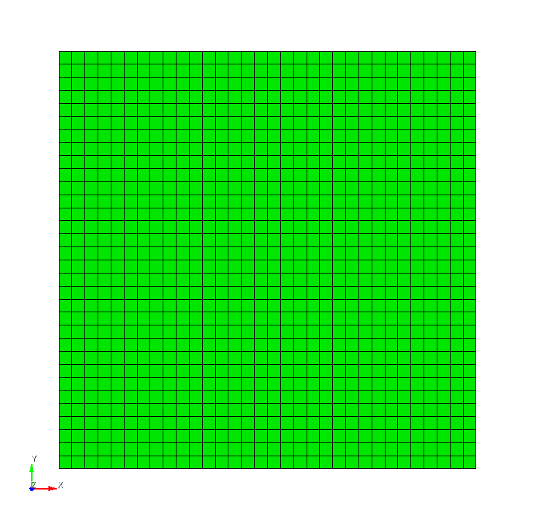
tutorial_scatra mesh — 2D mesh for the Poisson problem.

Five nodesets are defined in the exodus file. Node sets 1 to 4 represent the boundary lines. Node set 5 encompasses all nodes for the Neumann boundary condition.

In an exodus file, node sets may have names. Even though 4C does not utilize these names, they can be helpful for identifying sets. In the respective geometry input section, which depends on the analysis type (see here for scalar transport and here for the thermal analysis), one may print out the set names using the parameter SHOW_INFO: detailed_summary. The 4C output then contains a summary of the geometry, which is useful for verifying the mesh and node sets, see the relevant part here:

Mesh read in from "tutorial_poisson_geo.e"
  consists of 1089 Nodes and 1024 Elements;
  organized in 1 ElementBlocks, 5 NodeSets and 0 SideSets.

ElementBlocks
-------------
Block 1: 1024 Elements of Shape quad4

NodeSets
--------
NodeSet 1: (xmax) contains 33 Nodes
NodeSet 2: (xmin) contains 33 Nodes
NodeSet 3: (ymin) contains 33 Nodes
NodeSet 4: (ymax) contains 33 Nodes
NodeSet 5: (wholesurf) contains 1089 Nodes

We solve the system using the direct solver UMFPACK for simplicity. This is a robust serial solver that does not support MPI parallelization. However, for this small problem, parallelization or iterative solvers would not offer a performance benefit.

Boundary and Source Conditions

For both solver types, the boundary condition defines the primary variable (\(T\) or \(C\)) to be zero at the boundary. This corresponds to a Dirichlet condition applied to all four boundary lines and is identical in both cases:

DESIGN LINE DIRICH CONDITIONS:
- E: 1
  ENTITY_TYPE: node_set_id
  NUMDOF: 1
  ONOFF:
  - 1
  VAL:
  - 0.0
  FUNCT:
  - 0
- E: 2
  ENTITY_TYPE: node_set_id
  NUMDOF: 1
  ONOFF:
  - 1
  VAL:
  - 0.0
  FUNCT:
  - 0
- E: 3
  ENTITY_TYPE: node_set_id
  NUMDOF: 1
  ONOFF:
  - 1
  VAL:
  - 0.0
  FUNCT:
  - 0
- E: 4
  ENTITY_TYPE: node_set_id
  NUMDOF: 1
  ONOFF:
  - 1
  VAL:
  - 0.0
  FUNCT:
  - 0

The source term is constant throughout the domain, representing the right-hand side of the equation. This is implemented as a Neumann (flux) condition:

DESIGN SURF NEUMANN CONDITIONS:
- E: 5
  ENTITY_TYPE: node_set_id
  NUMDOF: 1
  ONOFF:
  - 1
  VAL:
  - 1.0
  FUNCT:
  - 0

Simulation is performed in a single load step for both problem types. Note that the initial conditions are irrelevant for steady-state simulations. However, for a time-dependent simulation, you would need to define an initial condition, i.e., an initial concentration or temperature.

Poisson Problem Solved with the Scalar Transport Solver

As mentioned earlier, the diffusion problem is treated as a scalar transport problem in 4C. Therefore, the PROBLEM TYPE section is set to Scalar_Transport, which determines the structure of most other sections in the input file and is thus particularly important:

PROBLEM TYPE:
  PROBLEMTYPE: Scalar_Transport

The time stepping and steady-state configuration are defined in the SCALAR TRANSPORT DYNAMIC section. Although the time step is irrelevant for a steady-state simulation, a value for TIMESTEP must still be provided. The simulation runs in a single step, so NUMSTEP: 1 is used. The solver is selected via LINEAR_SOLVER: 1, which refers to the corresponding SOLVER 1 section. The NAME parameter in the solver section is optional and can be any string.

SCALAR TRANSPORT DYNAMIC:
  TIMEINTEGR: Stationary
  TIMESTEP: 1
  MAXTIME: 1
  NUMSTEP: 1
  LINEAR_SOLVER: 1
SOLVER 1:
  SOLVER: UMFPACK
  NAME: direct linear solver

The only material parameter in this model is the diffusivity, which is defined in the MATERIALS section:

MATERIALS:
- MAT: 1
  MAT_scatra:
    DIFFUSIVITY: 1.0

The geometry, defined in the Exodus file (see above), is read using:

TRANSPORT GEOMETRY:
  ELEMENT_BLOCKS:
  - ID: 1
    TRANSP:
      QUAD4:
        MAT: 1
        TYPE: Std
  FILE: tutorial_poisson_geo.e
  SHOW_INFO: detailed_summary

In the ELEMENT_BLOCK section, the cell type, material, and transport formulation (here: Standard, denoted as Std) are specified.

For scalar transport simulations, the primary variable is written to VTK files as phi_1. Currently, the flux is not included in the VTK output. Therefore, no explicit output section is required in this input file.

Poisson Problem Solved with the Thermal Solver

Similar to the scalar transport solveer, the PROBLEM TYPE section - this time set to Thermo - defines the sections for the thermal solver to be used in the input file:

PROBLEM TYPE:
  PROBLEMTYPE: Thermo

The steady-state configuration is declared in the THERMAL DYNAMIC section. Unlike scalar transport, the steady-state condition is specified using DYNAMICTYPE: Statics. Again, the same direct linear solver is used.

THERMAL DYNAMIC:
  DYNAMICTYPE: Statics
  TIMESTEP: 1
  NUMSTEP: 1
  MAXTIME: 1
  LINEAR_SOLVER: 1
SOLVER 1:
  SOLVER: UMFPACK
  NAME: direct linear solver

Thermal conduction models always require two material parameters: heat capacity and conductivity. Although heat capacity is not relevant for steady-state simulations, both parameters must be defined:

MATERIALS:
- MAT: 1
  MAT_Fourier:
    CAPA: 1.0
    CONDUCT:
      constant:
      - 1.0

The geometry is read from the Exodus file using:

THERMO GEOMETRY:
  ELEMENT_BLOCKS:
  - ID: 1
    THERMO:
      QUAD4:
        MAT: 1
  FILE: tutorial_poisson_geo.e
  SHOW_INFO: detailed_summary

The ELEMENT_BLOCK section then defines the cell type and material.

Unlike scalar transport, thermal simulations do not produce VTK output unless explicitly requested. To enable output, the following two sections must be included:

IO/RUNTIME VTK OUTPUT:
  INTERVAL_STEPS: 1
THERMAL DYNAMIC/RUNTIME VTK OUTPUT:
  OUTPUT_THERMO: true
  TEMPERATURE: true

In addition to temperature, you may also choose to output conductivity (useful if it’s not constant), heat flux, and temperature gradient.

Post-Processing

After running either simulation, you can load the resulting .pvd file into ParaView. You can visualize the primary variable (phi_1 or temperature) on the surface, or apply the Warp by Scalar filter. By default, the structure is displayed in the x-y plane, so warping (which occurs in the z-direction) is not immediately visible. To view the deformation, rotate the structure accordingly.

The thermal simulation results are shown in the Warp plot (aka relief plot) below. The scalar transport results are nearly identical and are therefore omitted.

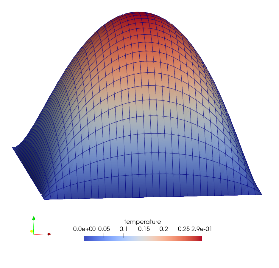
Scalar transport tutorial result relief of phi_1 — Relief plot of temperature from the thermal simulation. The scalar transport solution is visually identical, as is the result from the deal.II tutorial.

For comparison, we generate an x-y plot of the primary variables from both simulations along a path at \(y=0\). These results can be compared with deal.II tutorial step 3. Since the mesh is identical, the evaluated paths are indistinguishable.

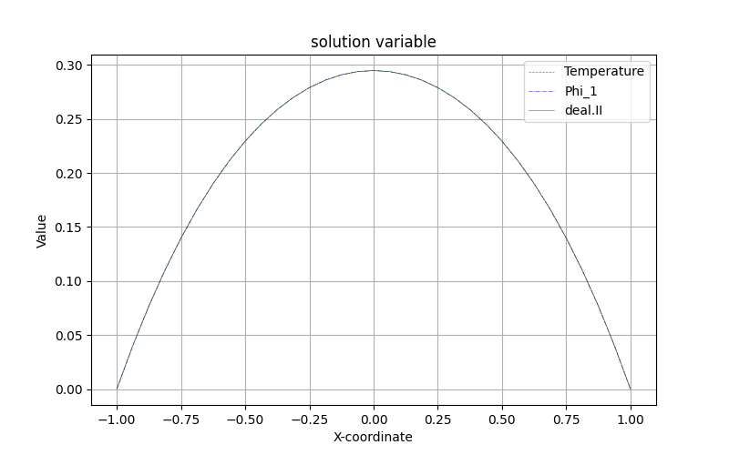
Poisson tutorial result graph at y=0 — Results along a line through the structure at \(y=0\) (center).

The error between the scalar transport and thermal conduction simulations is below \(10^{-14}\). The deal.II tutorial uses an iterative solver (conjugate gradient) with a tolerance of \(10^{-6}\). Thus, the error between the 4C and deal.II solutions is within this range, as shown below:

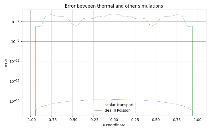
Error between deal.ii and thermal simulation — Error between diffusion and thermal conduction, and between deal.II and thermal conduction along the line at \(y=0\).

Here is a ParaView Python script <https://github.com/4C-multiphysics/4C/blob/main/utilities/four_c_python/src/four_c_documentation/tutorial_poisson_pvscript.py> that generates the figure for the structure loaded in ParaView (visible in Paraview’s current RenderView).