Tutorial: Preconditioners for Iterative Solvers

Preconditioners are a key tool to accelerate iterative solvers for large linear systems, improving convergence and robustness. From a theoretical perspective, they can be understood as transformations that reduce the condition number of the system matrix, thereby making iterative methods converge more rapidly.

For a broader, theoretical introduction to iterative methods and preconditioning, see Saad’s Iterative Methods for Sparse Linear Systems [1] among many others. Multiple sources for a theoretical background on Multigrid Methods can be found in literature, e.g., in Briggs et al., A Multigrid Tutorial [2] or many others. For an introduction to the use of linear solvers in 4C, we refer to this overview.

Note

In practical applications, the primary performance metric for simulation engineers is usually computation time rather than iteration counts. However, in this tutorial we deliberately focus on iteration counts: the small problem sizes chosen here make timing results unreliable and not representative. In contrast to timings, iteration counts are reproducible across problem sizes, hardware platforms and software configurations. For realistic, large-scale problems, timings are of course essential, but for illustrative purposes iteration counts are the more meaningful measure.

Overview

1. Solid mechanics: Solving linear systems arising from 3D elasticity

   1. Problem Setup

   2. Preliminary Steps

   3. Step 0: Iterative Solver without any Preconditioner

   4. Step 1: Iterative Solver with Jacobi preconditioner

   5. Step 2: Iterative Solver with Chebyshev preconditioner

   6. Step 3: Iterative Solver with Incomplete-LU Factorization Preconditioner

   7. Step 4: Iterative Solver with Smoothed-Aggregation Algebraic Multigrid Preconditioner

   8. Step 5: Indication of Weak Scaling Behavior

2. Block preconditioning of monolithic FSI solvers

   1. Step 1: Block-Iterative Preconditioner

   2. Step 2: Fully coupled Preconditioner

Solid mechanics: Solving linear systems arising from 3D elasticity

The following instructions will guide you through different preconditioner options to solve a linear system

\[ A x = b \]

arising from the finite element discretization of a cantilever beam using solid elements.

Problem Setup

Note

The exact details of the problem setup are not important for the course of this tutorial and, thus, are only summarized briefly.

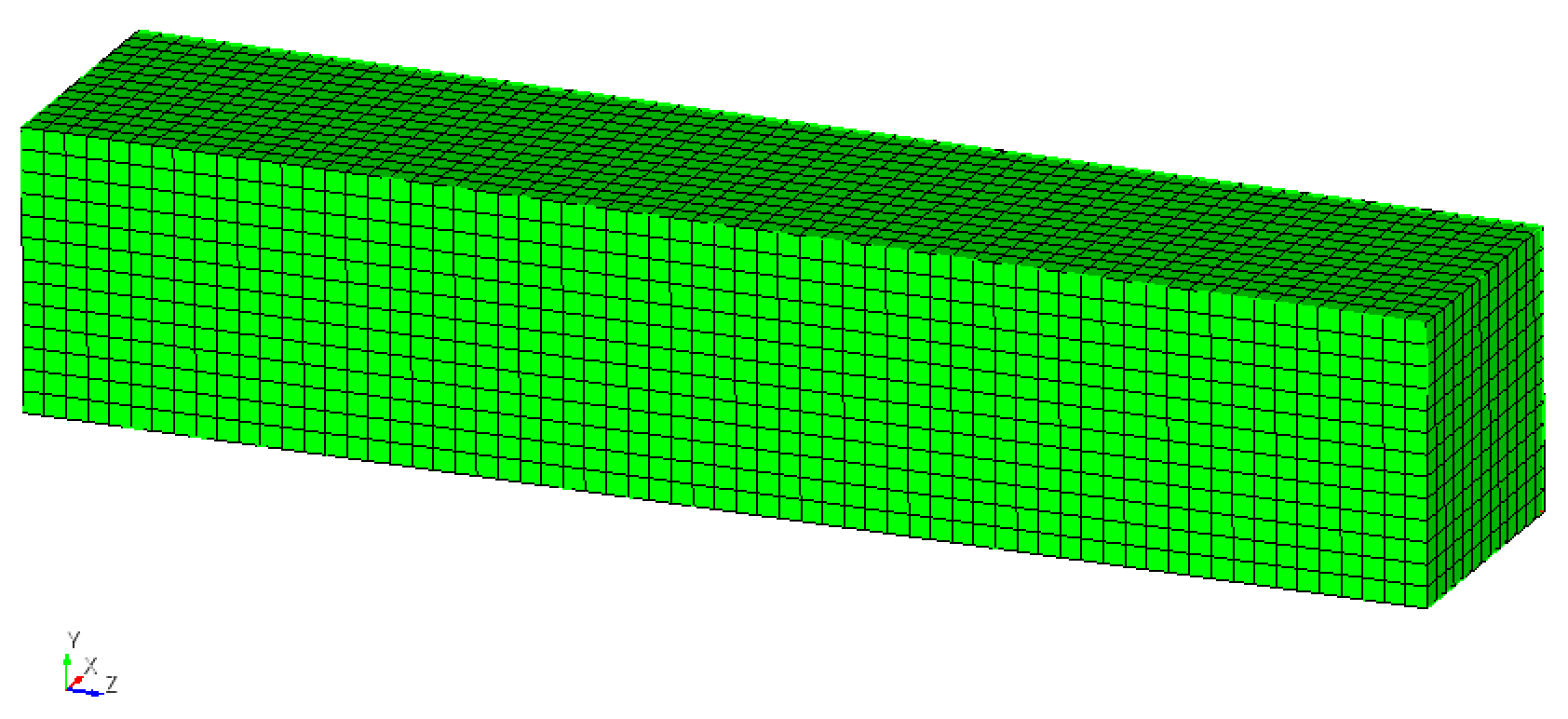
The problem consists of a cantilever beam with dimensions \(1 \times 1 \times 5\). It is fully clamped at \(z=0\). The surface at \(z=5\) is subject to a Dirichlet boundary condition, prescibing a displacement of \([0.01, 0.01, 0.01]\) in \([x, y, z]\) directions, respectively. A St.-Venant-Kirchhoff material with a Young’s modulus of \(1\) and a Poisson’s ration of \(0.3\) is used in combination with linear kinematics. The problem is configured to only solve a single linear system.

The geometry (with “mesh 1” defined below) looks as follows:

The simulation model with three possible meshes is defined using the following files:

• tutorial_prec_solid.4C.yaml: simulation parameters and boundary conditions for clamped cantilever beam with endload performing a single solve of the linear system

• tutorial_prec_solid_gmres.xml: definition of a GMRES solver from Belos (required for iterative solvers throughout the tutorial)

• a series of mesh files tutorial_prec_solid_*.exo to change the size of the linear system to be solved (see table with meshing details)

Meshing details:

Mesh file	#nodes x	#nodes y	#nodes z	#DOFs	#MPI ranks
tutorial_prec_solid_0.exo	3	3	15	405	1
tutorial_prec_solid_1.exo	12	12	60	25920	1
tutorial_prec_solid_2.exo	16	16	80	61440	2
tutorial_prec_solid_3.exo	20	20	100	120000	4
tutorial_prec_solid_4.exo	23	23	115	182505	6
tutorial_prec_solid_5.exo	25	25	125	234375	8

Different preconditioners are predefined in the following files:

• tutorial_prec_solid_ifpack_Jacobi.xml

• tutorial_prec_solid_ifpack_Chebyshev.xml

• tutorial_prec_solid_ifpack_ILU.xml

• tutorial_prec_solid_muelu_sa_amg.xml

They will be used and modified throughout this tutorial.

Note

Remark: choice of input parameters

Since this tutorial focuses on preconditioning of the linear solver, we are not really interested in solving an actual solid mechanics problem, but only want to solve a single linear system arising from solid mechanics. To do this in 4C, the time integration just performs one step (cf. NUMSTEP: 1), the nonlinear solver is limited to one iteration by setting MAXITER: 1. Nonlinear solver tolerances are chosen very loosely, such that the nonlinear solver assumes convergence after one step.

These are artifical settings for the purpose of this tutorial. They do not serve as a recommendation for any meaningful simulation in 4C.

Preliminary Steps

The default input file comes with a direct solver, so you can run it right away. To run it on <numProc> MPI ranks, use the following command:

mpirun -np <numProcs> <4Cexe> tutorial_prec_solid.4C.yaml output

Please verify, that the simulation has finished successfully.

Step 0: Iterative Solver without any Preconditioner

In theory, you can run a Krylov solver without any preconditioner and it will converge in \(N\) iterations for a system with \(N\) equations. Since unpreconditioned Krylov solvers are known to deliver bad performance [1], 4C does not offer this option, and we also do not cover it in this tutorial.

Step 1: Iterative Solver with Jacobi preconditioner

The tutorial_prec_solid.4C.yaml input file comes with a pre-configured iterative solver (GMRES) with a relaxation preconditioner, namely Jacobi’s method. In the input file, it is defined in SOLVER 2. The preconditioner is configured in the file tutorial_prec_solid_ifpack_Jacobi.xml.

To switch to GMRES with a Jacobi preconditioner, set the solid LINEAR_SOLVER to 2.

1. Open the tutorial_prec_solid.4C.yaml input file.

2. Familiarize yourself with the list SOLVER 2 and the file tutorial_prec_solid_ifpack_Jacobi.xml.

3. To switch to the new solver,

   1. find the list STRUCTURAL DYNAMIC,

   2. modify the value of its parameter LINEAR_SOLVER to 2.

4. Save the file tutorial_prec_solid.4C.yaml

Solution

STRUCTURAL DYNAMIC:
  INT_STRATEGY: Standard
  DYNAMICTYPE: Statics
  TIMESTEP: 1.0
  NUMSTEP: 1
  MAXTIME: 1
  MAXITER: 1
  RESULTSEVERY: 0
  RESTARTEVERY: 0
  NORMCOMBI_RESFDISP: Or
  DIVERCONT: continue
  LINEAR_SOLVER: 2

Now, run the example and watch the convergence behavior of the iterative solver.

Note

Where to find the number of GMRES iterations?

For this tutorial, 4C is configured to only perform a single Newton step, such that you can really focus on the solution of a single linear system of equations. By default, the iterative solver will output residual information in every iteration.

The setup and solution process of the linear solver produce output similar to this:

*******************************************************
***** Belos Iterative Solver:  Pseudo Block Gmres
***** Maximum Iterations: 2000
***** Block Size: 1
***** Status tests:
   Failed.......OR Combination ->
     OK...........Number of Iterations = 0 < 2000
     Unconverged..(2-Norm Res Vec) / (2-Norm Prec Res0)
                  residual [ 0 ] = 1.000000e+00 > 1.000000e-10

*******************************************************
           [ 1] :    IMPLICIT RES
Iter    0, [ 1] :    1.000000e+00
Iter    1, [ 1] :    2.987968e-02
Iter    2, [ 1] :    4.747745e-03
Iter    3, [ 1] :    4.079741e-04
Iter    4, [ 1] :    5.292770e-05
Iter    5, [ 1] :    9.309950e-06
Iter    6, [ 1] :    1.418433e-06
Iter    7, [ 1] :    2.224382e-07
Iter    8, [ 1] :    3.003654e-08
Iter    9, [ 1] :    3.225869e-09
Iter   10, [ 1] :    3.924956e-10
Iter   11, [ 1] :    4.445936e-11

The linear solver tolerance is set to 1e-10, such that in this output the line

Iter   11, [ 1] :    4.445936e-11

shows the last iteration of the linear solver. From there, you can conclude that the linear solver required 11 iterations until convergence.

Study the influence of the following parameters on the number of GMRES iterations and/or runtime until convergence:

• Configuration of the preconditioner:

  • Number of sweeps: "relaxation: sweeps" [Range: 1 - 5]

  • Number of sweeps: "relaxation: damping factor" [Range: 0.1 - 1.0]

• Mesh (to be set in tutorial_prec_solid.4C.yaml)

  • tutorial_prec_solid_1.exo (for 1 MPI process)

  • tutorial_prec_solid_2.exo (for 2 MPI processes)

  • tutorial_prec_solid_3.exo (for 4 MPI processes)

  • tutorial_prec_solid_4.exo (for 6 MPI processes)

  • tutorial_prec_solid_5.exo (for 8 MPI processes)

Expected outcome

• More sweeps reduce the number of iterations.

• Smaller damping values, i.e., more damping, increase the number of iterations.

Step 2: Iterative Solver with Chebyshev preconditioner

The tutorial_prec_solid.4C.yaml input file comes with a pre-configured iterative solver (GMRES) with a polynomial preconditioner using Chebyshev polynomials. In the input file, it is defined in SOLVER 3. The preconditioner is configured in the file tutorial_prec_solid_ifpack_Chebyshev.xml.

To switch to GMRES with a Chebyshev preconditioner, set the solid LINEAR_SOLVER to 3.

Solution

STRUCTURAL DYNAMIC:
  INT_STRATEGY: Standard
  DYNAMICTYPE: Statics
  TIMESTEP: 1.0
  NUMSTEP: 1
  MAXTIME: 1
  MAXITER: 1
  RESULTSEVERY: 0
  RESTARTEVERY: 0
  NORMCOMBI_RESFDISP: Or
  DIVERCONT: continue
  LINEAR_SOLVER: 3

Now, run the example and watch the convergence behavior of the iterative solver. Study the influence of the following parameters on the number of GMRES iterations and/or runtime until convergence:

• Configuration of the preconditioner:

  • Polynomial degree: "chebyshev: degree" [Range: 1 - 6]

• Mesh (to be set in tutorial_prec_solid.4C.yaml)

  • tutorial_prec_solid_1.exo (for 1 MPI process)

  • tutorial_prec_solid_2.exo (for 2 MPI processes)

  • tutorial_prec_solid_3.exo (for 4 MPI processes)

  • tutorial_prec_solid_4.exo (for 6 MPI processes)

  • tutorial_prec_solid_5.exo (for 8 MPI processes)

Expected outcome

Larger polynomial degrees reduce the number of iterations.

Step 3: Iterative Solver with Incomplete-LU Factorization Preconditioner

The tutorial_prec_solid.4C.yaml input file comes with a pre-configured iterative solver (GMRES) with an incomplete LU factorization (ILU) preconditioner. In the input file, it is defined in SOLVER 4. The preconditioner is configured in the file tutorial_prec_solid_ifpack_ILU.xml.

To switch to GMRES with an ILU preconditioner, set the solid LINEAR_SOLVER to 4.

Solution

STRUCTURAL DYNAMIC:
  INT_STRATEGY: Standard
  DYNAMICTYPE: Statics
  TIMESTEP: 1.0
  NUMSTEP: 1
  MAXTIME: 1
  MAXITER: 1
  RESULTSEVERY: 0
  RESTARTEVERY: 0
  NORMCOMBI_RESFDISP: Or
  DIVERCONT: continue
  LINEAR_SOLVER: 4

Now, run the example and watch the convergence behavior of the iterative solver. Study the influence of the following parameters on the number of GMRES iterations and/or runtime until convergence:

• Configuration of the preconditioner:

  • Overlap at processor boundaries: "Overlap" defines the overlap at processor boundaries (0 = no overlap, larger values results in larger overlap) [Range: 0 - 2]

  • Fill-in: "fact: level-of-fill" defines the allowed fill-in (larger values result in a better approximation, however a more expensive setup procedure) [Range: 0 - 3]

• Mesh (to be set in tutorial_prec_solid.4C.yaml)

  • tutorial_prec_solid_1.exo (for 1 MPI process)

  • tutorial_prec_solid_2.exo (for 2 MPI processes)

  • tutorial_prec_solid_3.exo (for 4 MPI processes)

  • tutorial_prec_solid_4.exo (for 6 MPI processes)

  • tutorial_prec_solid_5.exo (for 8 MPI processes)

Expected outcome

Larger fill-in reduces the number of iterations, but increases the preconditioner setup time.

Step 4: Iterative Solver with Smoothed-Aggregation Algebraic Multigrid Preconditioner

The tutorial_prec_solid.4C.yaml input file comes with a pre-configured iterative solver (GMRES) with a smoothed aggregation algebraic multigrid preconditioner. In the input file, it is defined in SOLVER 5. The preconditioner is configured in the file tutorial_prec_solid_muelu_sa_amg.xml.

To switch to GMRES with an algebraic multigrid preconditioner, set the solid LINEAR_SOLVER to 5.

Solution

STRUCTURAL DYNAMIC:
  INT_STRATEGY: Standard
  DYNAMICTYPE: Statics
  TIMESTEP: 1.0
  NUMSTEP: 1
  MAXTIME: 1
  MAXITER: 1
  RESULTSEVERY: 0
  RESTARTEVERY: 0
  NORMCOMBI_RESFDISP: Or
  DIVERCONT: continue
  LINEAR_SOLVER: 5

Now, run the example and watch the convergence behavior of the iterative solver. Study the influence of the following parameters on the number of GMRES iterations and/or runtime until convergence:

• Configuration of the preconditioner:

  • Polynomial degree of the Chebyshev level smoother: "chebyshev: degree" [Range: 0 - 6]

• Mesh (to be set in tutorial_prec_solid.4C.yaml)

  • tutorial_prec_solid_1.exo (for 1 MPI process)

  • tutorial_prec_solid_2.exo (for 2 MPI processes)

  • tutorial_prec_solid_3.exo (for 4 MPI processes)

  • tutorial_prec_solid_4.exo (for 6 MPI processes)

  • tutorial_prec_solid_5.exo (for 8 MPI processes)

Expected outcome

Larger polynomial degrees reduce the number of iterations.

If you like to investigate a different level smoother, follow the “Optional study: change the level smoother”.

Optional study: change the level smoother

1. Open the preconditioner configuration tutorial_prec_solid_muelu_sa_amg.xml

2. Comment the list of the Chebyshev level smoother and uncomment the list of the Gauss-Seidel level smoother

   <!-- ===========  SMOOTHING  =========== -->
   <!--<Parameter name="smoother: type" type="string" value="CHEBYSHEV"/>
   <ParameterList name="smoother: params">
     <Parameter name="chebyshev: degree" type="int" value="4"/>
     <Parameter name="chebyshev: ratio eigenvalue" type="double" value="7"/>
     <Parameter name="chebyshev: min eigenvalue" type="double" value="1.0"/>
     <Parameter name="chebyshev: zero starting solution" type="bool" value="true"/>
   </ParameterList>-->
   <Parameter name="smoother: type" type="string" value="RELAXATION"/>
   <ParameterList name="smoother: params">
     <Parameter name="relaxation: type" type="string" value="Gauss-Seidel"/>
     <Parameter name="relaxation: sweeps" type="int" value="1"/>
     <Parameter name="relaxation: damping factor" type="double" value="1.0"/>
   </ParameterList>
   

3. Run the example, study the effect of different Gauss-Seidel parameters on the number of GMRES iterations and/or runtime until convergence.

Expected outcome:

• More sweeps reduce the number of iterations.

• Smaller damping values, i.e., more damping, increase the number of iterations.

Step 5: Indication of Weak Scaling Behavior

We now compare the iteration counts of different preconditioners to indicate weak scaling behavior. Due to its practical relevance, we study weak scaling behavior [3], i.e., we increase the problem size at the same rate as the computing resources yielding a constant load (number of unknowns) per MPI process and expect a constant performance of the iterative solver.

For the purpose of this tutorial, we assess the performance by the number of GMRES iterations required to reach convergence. For simplicity, we refrain from assessing timings in this tutorial.

To assess the iteration count of a particular preconditioner, perform the following steps:

1. Select a preconditioner by choosing one of the predefined SOLVERs in tutorial_prec_solid.4C.yaml.

   1. Choose a parametrization for this preconditioner in the respective tutorial_prec_solid_*.xml file (and keep it constant for the entire study)

   2. Study one mesh

      1. Select a mesh by setting tutorial_prec_solid_*.exo in the input file.

      2. Run the example using the suitable number of MPI processes (as listed in the table on meshing details)

      3. Take a note of the number of GMRES iterations required to reach convergence

   3. Study the next mesh (i.e., repeat step ii with another mesh until all meshes have been computed.)

2. Go to step 1 and select a different preconditioner

Note

Make sure to at least cover one of the preconditioners from Ifpack and the multigrid preconditioner from MueLu.

Think about this:

• How does the iteration count behave for a growing number of MPI processes and unknowns?

• What is the main difference between the multigrid preconditioner and all the other one-level preconditioners?

Comparison of Iteration Counts

The iteration counts of the following preconditioners are compared:

• Jacobi: 1 sweep with damping 1.0

• Chebyshev: polynomial degree 3

• ILU: fill-level 0

• SA-AMG: V-cycle with Chebyshev polynomials of degree 2 as level smoothers

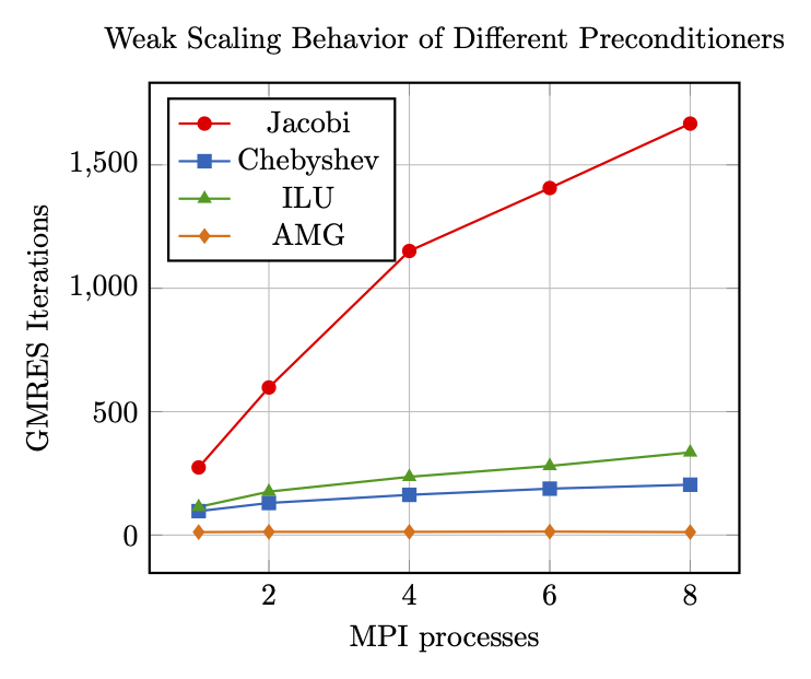
To make it reproducible on a laptop or desktop workstation, scaling behavior is assessed for 1, 2, 4, 6, and 8 MPI processes only. The number of iterations for each mesh and preconditioner are reported in the following figure:

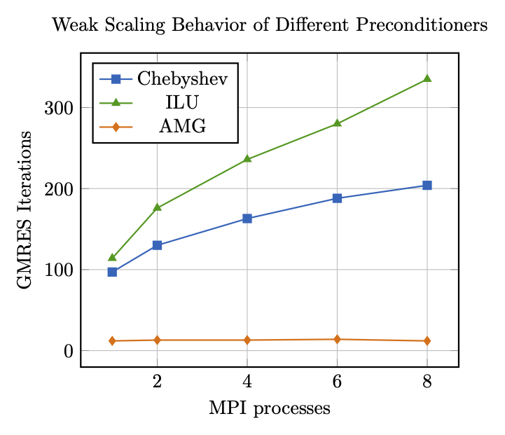
For a less distorted diagram, here is a plot of the same data without the Jacobi preconditioner:

Here are the numbers in detail:

Procs	1	2	4	6	8
Jacobi	274	598	1151	1406	1667
Chebyshev	97	130	163	188	204
ILU	114	176	236	280	335
AMG	12	13	13	14	12

It can clearly be seen, that

1. the multigrid preconditioner outperforms all other methods by far

2. the multigrid preconditioner is the only preconditioner indicating optimal weak scaling, i.e., the only one that delivers iteration counts independent of the problem size.

Block preconditioning of monolithic FSI solvers

We now study two different multilevel block preconditioning approaches[4] for monolithic fluid/solid interaction (FSI) solvers. As a test case, we use a pressure wave travelling through an elastic tube, which is often considered a standard benchmark for monolithic FSI solvers.

The arising linear system of equations exhibits \(3 \times 3\) block structure, reading[4],[5]:

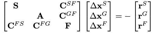
Note

A software implementation of monolithic FSI might use a different ordering of the fields. Again, the exact details of the problem setup are not important for the course of this tutorial and, thus, are omitted for the sake of brevity.

The simulation model is defined using the following files:

• tutorial_prec_fsi.4C.yaml: simulation parameters and boundary conditions for a pressure wave travelling through an elastic tube

• tutorial_prec_fsi_gmres.xml: definition of a GMRES solver from Belos (required for iterative solvers throughout the tutorial)

• tutorial_prec_fsi.exo: mesh in binary format

Different preconditioners are predefined in the following files:

• tutorial_prec_fsi_teko_block_iterative.xml

• tutorial_prec_fsi_muelu_fully_coupled_amg.xml

They will be used and modified throughout this tutorial.

Step 1: Block-Iterative Preconditioner

We first study a block-iterative preconditioner implemented via Teko[6]. Its configuration is given in tutorial_prec_fsi_teko_block_iterative.xml. It is defined as SOLVER 2 in the input file and is activated by default.

1. Open tutorial_prec_fsi_teko_block_iterative.xml and familiarize yourself with the file and its content.

   Some background on the file structure for Teko preconditioners

   The list Preconditioner defines the overall layout of the block preconditioner:

   <ParameterList name="Preconditioner">
     <Parameter name="Type" type="string" value="Block Gauss-Seidel"/>
     <Parameter name="Use Upper Triangle" type="bool" value="false"/>
     <Parameter name="Inverse Type 1" type="string" value="Inverse1"/>
     <Parameter name="Inverse Type 2" type="string" value="Inverse2"/>
     <Parameter name="Inverse Type 3" type="string" value="Inverse3"/>
   </ParameterList>
   

   In this case, it selects a Block Gauss-Seidel approach. Furthermore, it specifies names of lists (Inverse1, Inverse2, Inverse3) which provide details on how to approximate the necessary block inverses of the first, second, and third block within the \(3 \times 3\) block system.

   Then, an approximate inversion of each block is specified in their own sublists. For the solid block (Inverse1), this reads:

   <!-- ===========  SINGLE FIELD PRECONDITIONER FOR SOLID ================ -->
   <ParameterList name="Inverse1">
     <Parameter name="Type" type="string" value="MueLu"/>
     <Parameter name="multigrid algorithm" type="string" value="sa"/>
     <Parameter name="verbosity" type="string" value="None"/>
     <Parameter name="coarse: max size" type="int" value="200"/>
     <Parameter name="smoother: type" type="string" value="CHEBYSHEV"/>
     <ParameterList name="smoother: params">
       <Parameter name="chebyshev: degree" type="int" value="2"/>
       <Parameter name="chebyshev: min eigenvalue" type="double" value="1.0"/>
       <Parameter name="chebyshev: zero starting solution" type="bool" value="true"/>
     </ParameterList>
   </ParameterList>
   

   It uses MueLu with an sa (smoothed aggregation) algebraic multigrid scheme and provides all other parameters to properly define a MueLu hierarchy.

   Note

   This part might look familiar, as it just resembles a “standard” MueLu xml file as you have already seen it in the first part of this tutorial, where we have used MueLu for a solid mechanics problem.

   Analogously, sublists Inverse2 and Inverse3 define approximate inversions for the fluid and ALE block, respectively.

2. Run the example on two MPI processes via

   mpirun -np 2 <4Cexe> tutorial_prec_fsi.4C.yaml output
   

3. Study the influence of the preconditioner configuration on the number of GMRES iterations and/or runtime until convergence. Therefore, adapt the preconditioner settings in tutorial_prec_fsi_teko_block_iterative.xml.

Step 2: Fully coupled Preconditioner

Now, we switch to a fully coupled AMG preconditioner implemented in MueLu[7]. Its configuration is given in tutorial_prec_fsi_muelu_fully_coupled_amg.xml. It is defined as SOLVER 3 in the input.

1. Open the input file tutorial_prec_fsi.4C.yaml.

2. Find the section FSI DYNAMIC/MONOLITHIC SOLVER and set its parameter LINEAR_SOLVER to 3.

To study the preconditioner, perform the following steps:

1. Open tutorial_prec_fsi_muelu_fully_coupled_amg.xml and familiarize yourself with the file and its content.

   Some background on the file structure for MueLu block preconditioners

   MueLu block preconditioners can be defined via MueLu’s “advanced” input deck. This details all factories, i.e., building blocks of a multigrid hierarchy in sublists of the xml file. These are then processed by MueLu and stitched together to create a MueLu preconditioner.

   • The list Factories collects all individual factories. Factories can refer to other factories, e.g., for using the result of factory A as input for factory B. Therefore, factory A must be defined prior to factory B in the list of all factories. Other than that, the ordering of the factories is arbitrary. In this spirit, aggregation, transfer operators, or smoothers (or any other component of a MueLu hierarchy) are represented via their own sublist in the Factories list.

   • The list Hierarchy defines the actual multigrid hierarchy based on some parameters and the factories from above.

2. Run the example on two MPI processes via

   mpirun -np 2 <4Cexe> tutorial_prec_fsi.4C.yaml output
   

3. Study the influence of the preconditioner configuration on the number of GMRES iterations and/or runtime until convergence. Therefore, adapt the preconditioner settings in tutorial_prec_fsi_muelu_fully_coupled.xml. You could change the following components of the preconditioner:

   • Number of sweeps and damping parameter of the block Gauss-Seidel level smoother, cf. sublist myBlockSmoother

   • Polynomial degrees of Chebyshev smoothers for solid, fluid, ale blocks, cf. mySmooFact1, mySmooFact2, mySmooFact3

---

[1] (1,2)

Y. Saad. Iterative Methods for Sparse Linear Systems. SIAM, Philadelphia, PA, USA, 2003

[2]

W. L. Briggs, V. E. Henson, S. F. McCormick. A Multigrid Tutorial, 2nd Edition, Society for Industrial and Applied Mathematics, 2000

[3]

J. L. Gustafson. Reevaluating Amdahl’s law. Communications of the ACM, 31(5):532–533, 1988

[4] (1,2)

M. W. Gee, U. Küttler, and W. A. Wall. Truly monolithic algebraic multigrid for fluid–structure interaction. International Journal for Numerical Methods in Engineering, 85(8):987–1016, 2011

[5]

M. Mayr, T. Klöppel, W. A. Wall, and M. W. Gee. A Temporal Consistent Monolithic Approach to Fluid–Structure Interaction Enabling Single Field Predictors. SIAM Journal on Scientific Computing, 37(1):B30–B59, 2015

[6]

E. C. Cyr, J. N. Shadid, and R. S. Tuminaro. Teko: A Block Preconditioning Capability with Concrete Example Applications in Navier–Stokes and MHD. SIAM Journal on Scientific Computing, 38(5):S307–S331, 2016

[7]

L. Berger-Vergiat, C. A. Glusa, G. Harper, J. J. Hu, M. Mayr, A. Prokopenko, C. M. Siefert, R. S. Tuminaro, and T. A. Wiesner. MueLu User’s Guide. Technical Report SAND2023-12265, Sandia National Laboratories, Albuquerque, NM (USA) 87185, 2023